Control Systems · Part 1B

UR5e Controller Design, Benchmarking & Robustness

Building on the validated and characterized UR5e plant from Part 1A, I designed and evaluated PID, computed-torque, discrete LQR, and constrained MPC controllers on one common nonlinear benchmark. The study progresses beyond nominal tracking to diagnose controller-specific behavior, validate Python–C++ implementations, measure computation, and test robustness under persistent payload mismatch and a transient external disturbance.

UR5ePIDComputed TorqueLQRMPCRobustnessOSQPC++

View source on GitHub →

4Controller architectures on one common nonlinear benchmark

0.00124°Computed-torque nominal overall joint RMSE

2Robustness cases separating model mismatch and external disturbance

Engineering objective: compare controller assumptions and trade-offs rather than select a universal “best” controller. Nominal accuracy, robustness, computation, model dependence, and implementation behavior are evaluated separately.

1. Common Benchmark

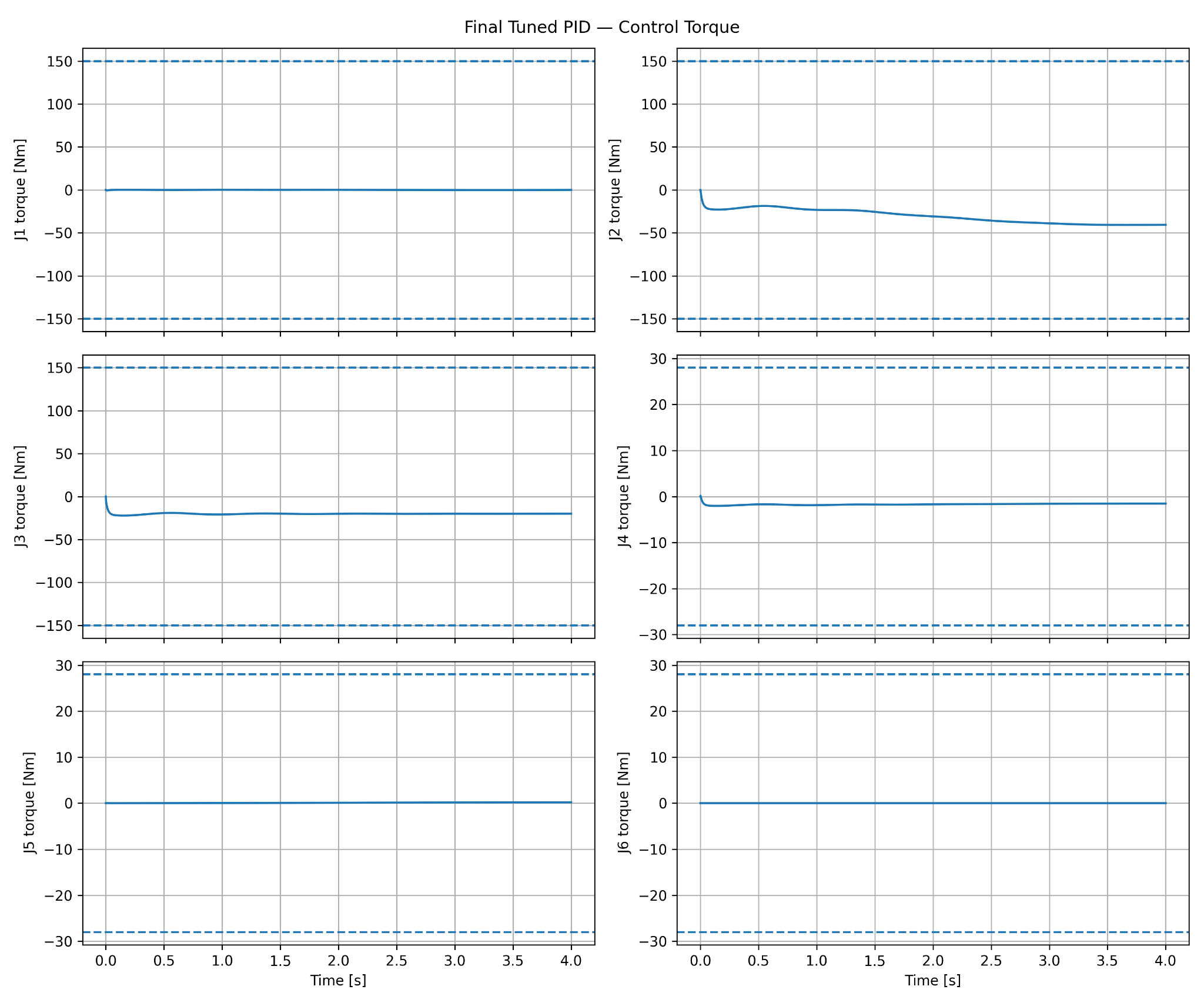
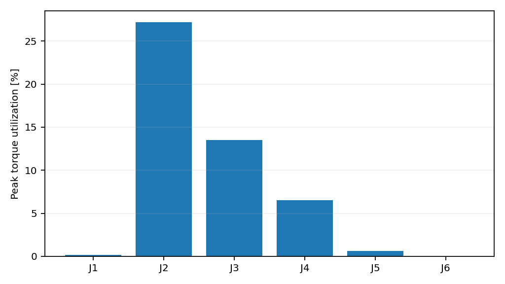
All controllers use the same validated nonlinear rigid-body plant, initial condition, reference trajectory, 2 ms sampling period, and modeled torque limits. The 4 s quintic trajectory moves from [0, -90, 90, -90, -90, 0]° to [20, -60, 60, -70, -70, 20]°. Part 1A established that this trajectory is dynamically meaningful without being saturation dominated.

Controller	Joint RMSE	TCP Position RMSE	TCP Orientation RMSE
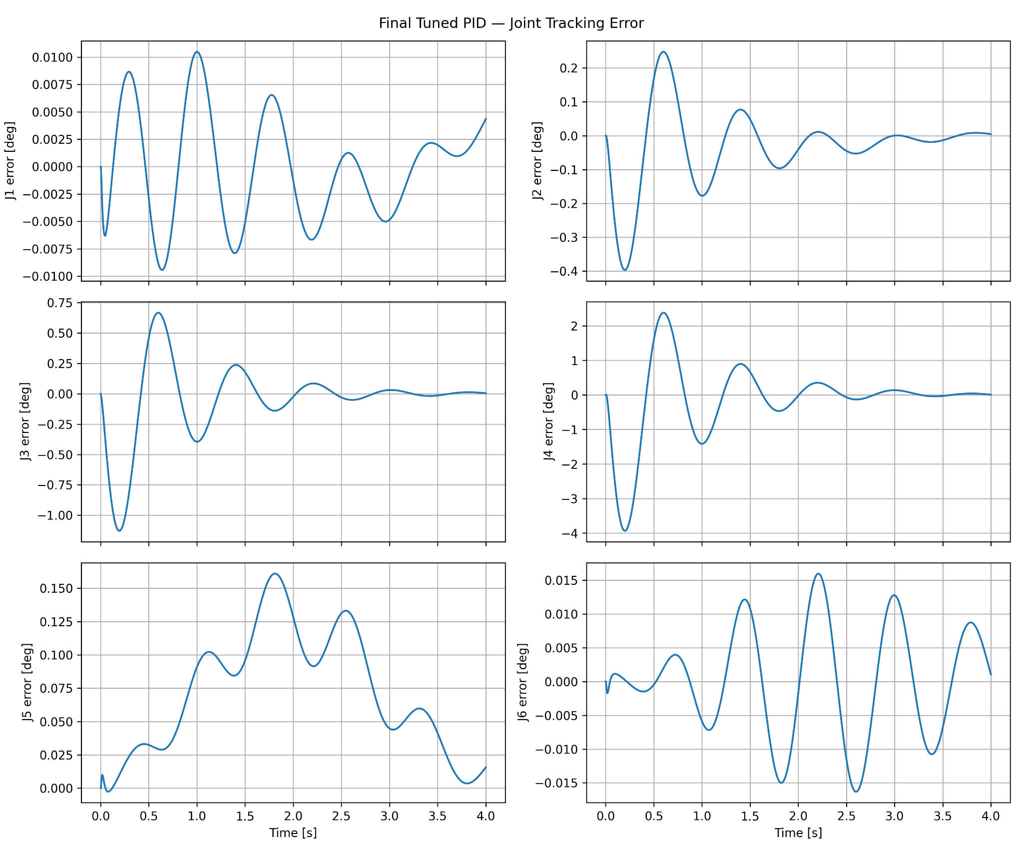
PID	0.469844°	5.835795 mm	1.527910°
Computed Torque	0.001244°	0.004139 mm	0.002883°
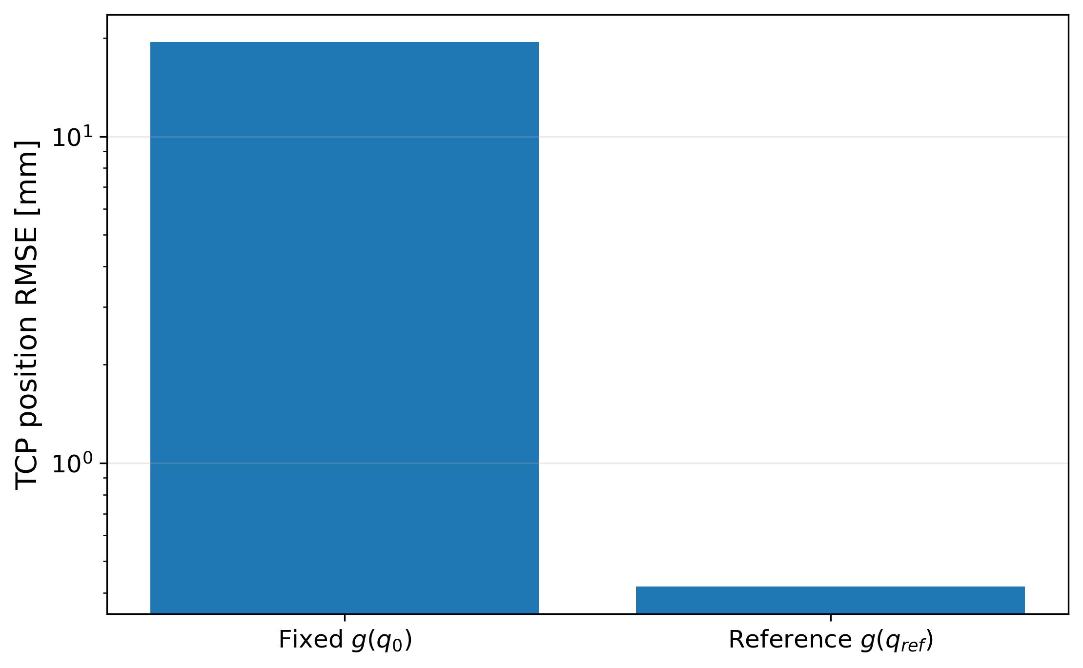
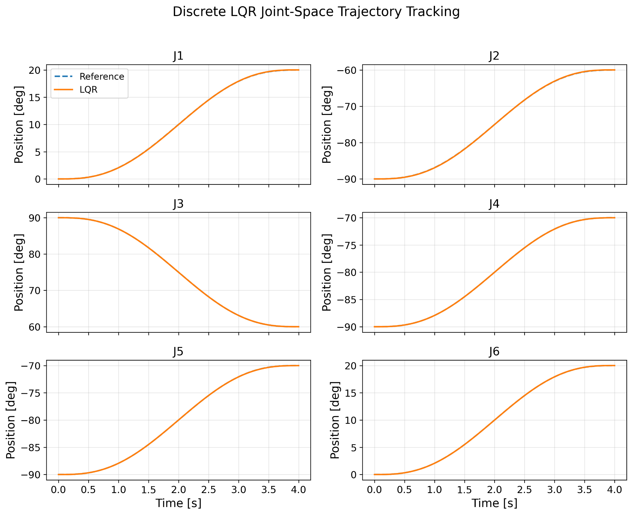
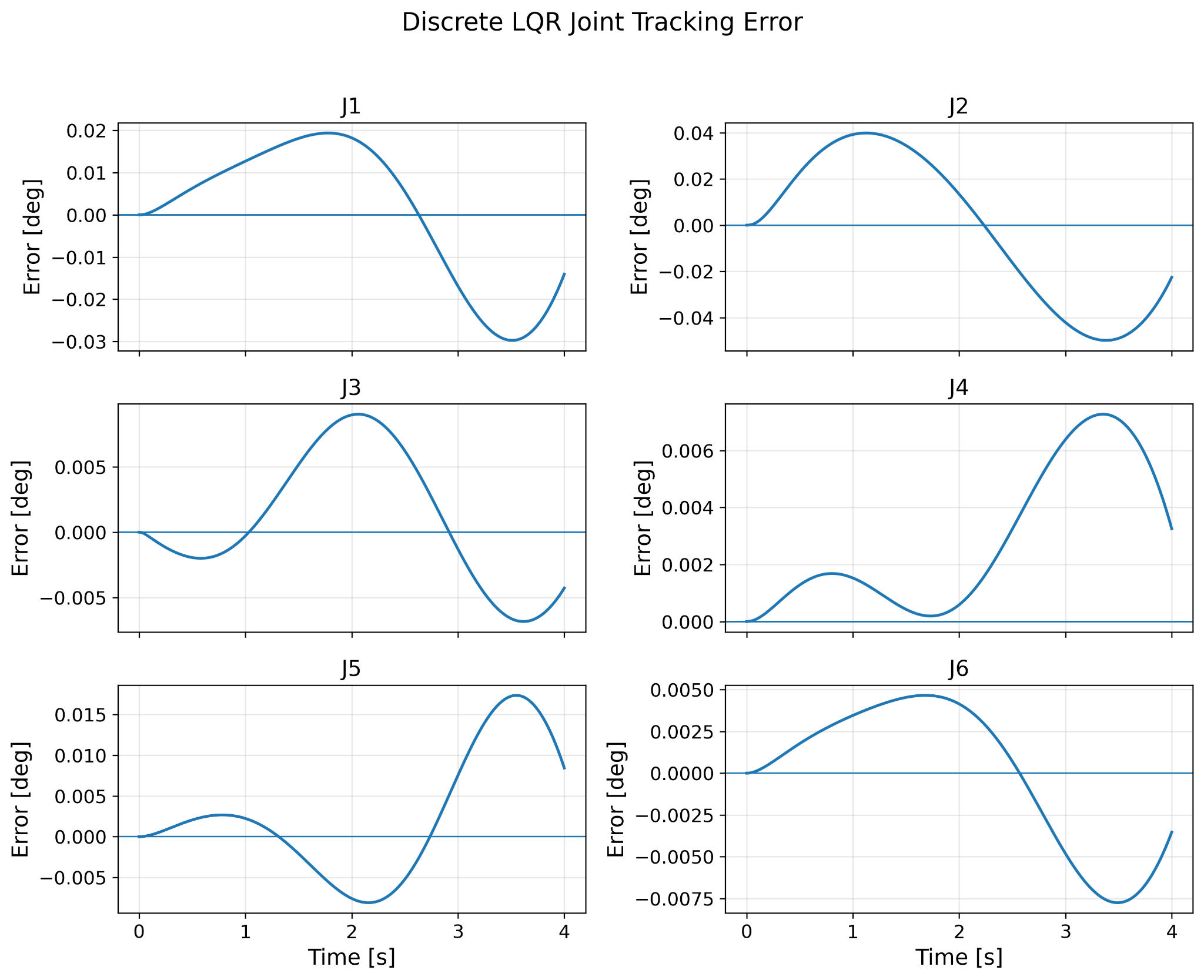
LQR	0.015502°	0.418511 mm	0.037763°
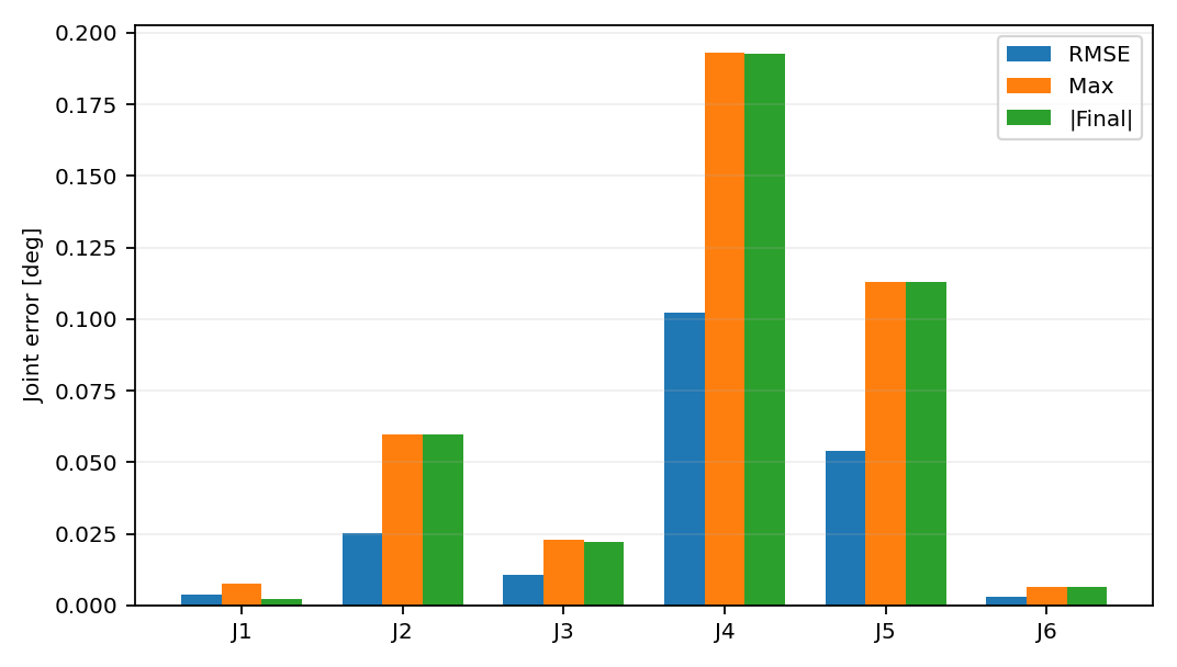
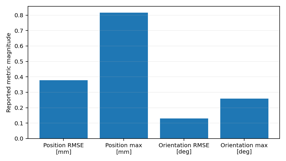
MPC	0.048474°	0.378424 mm	0.129772°

2. PID — Feedback Baseline and Dynamic Diagnosis

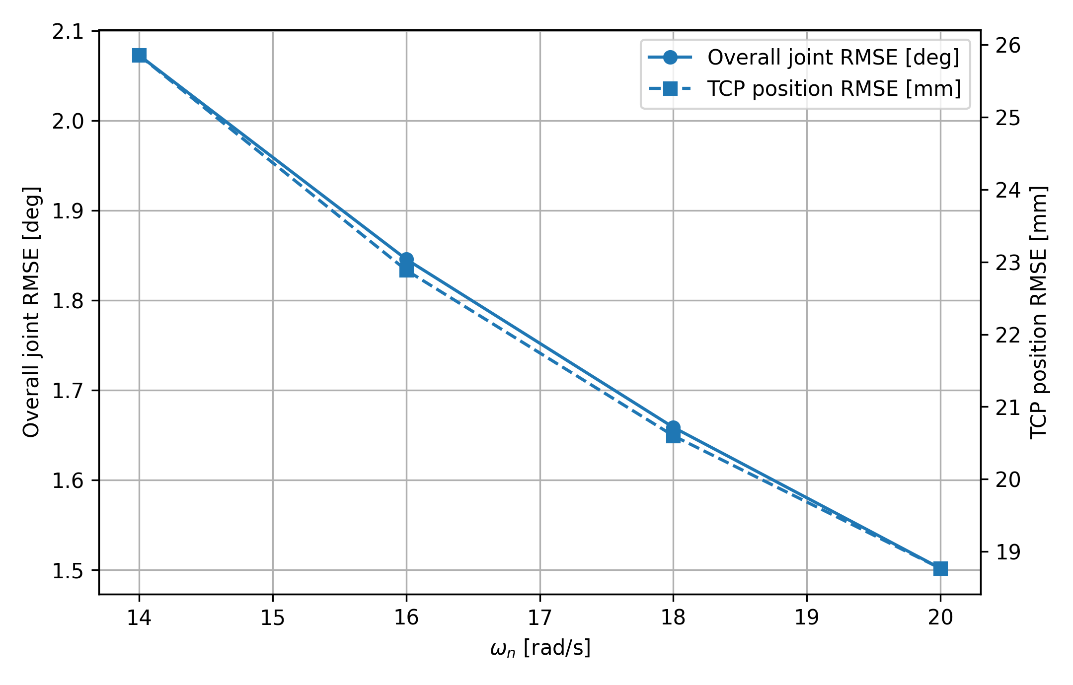
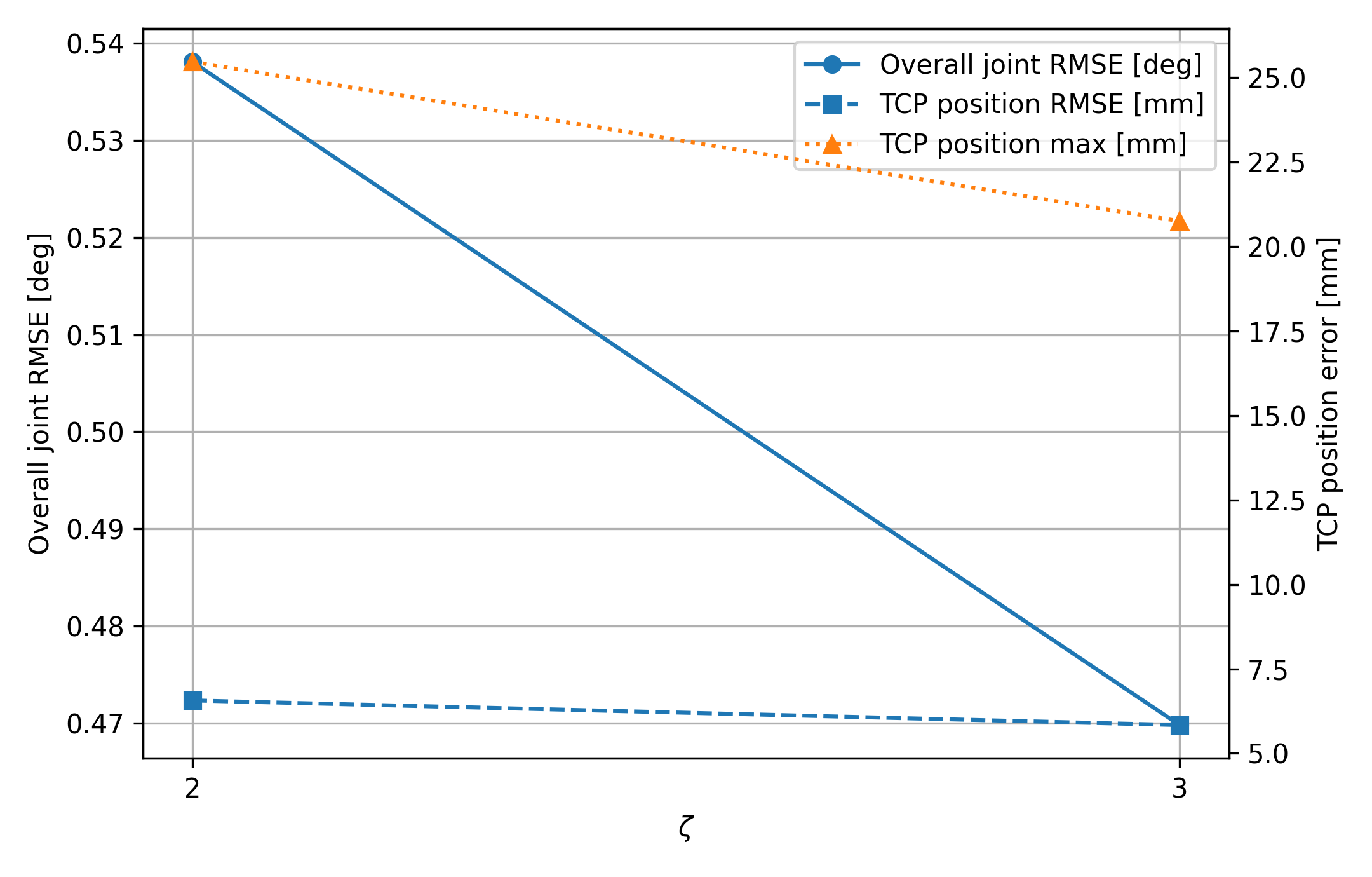
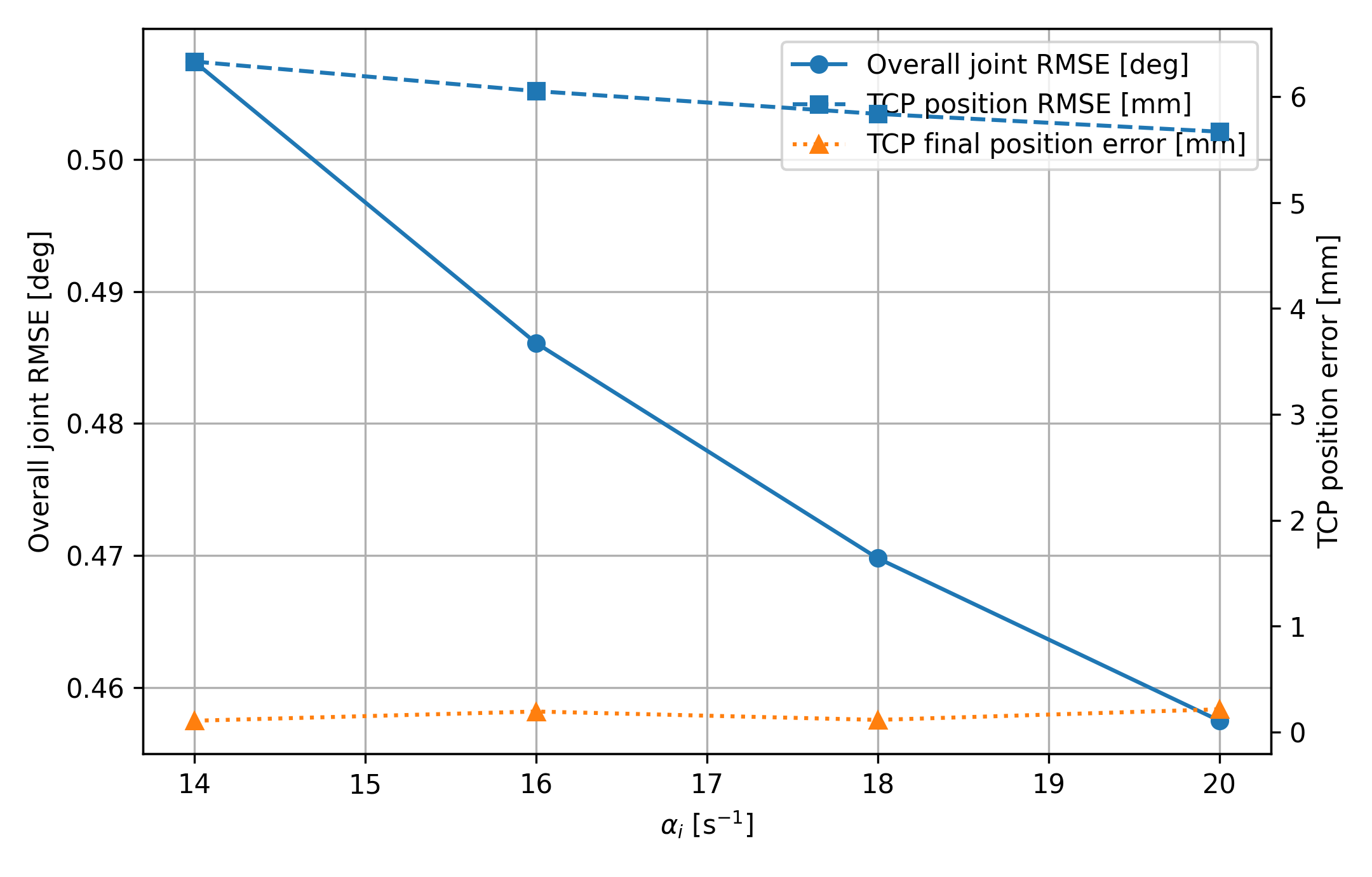
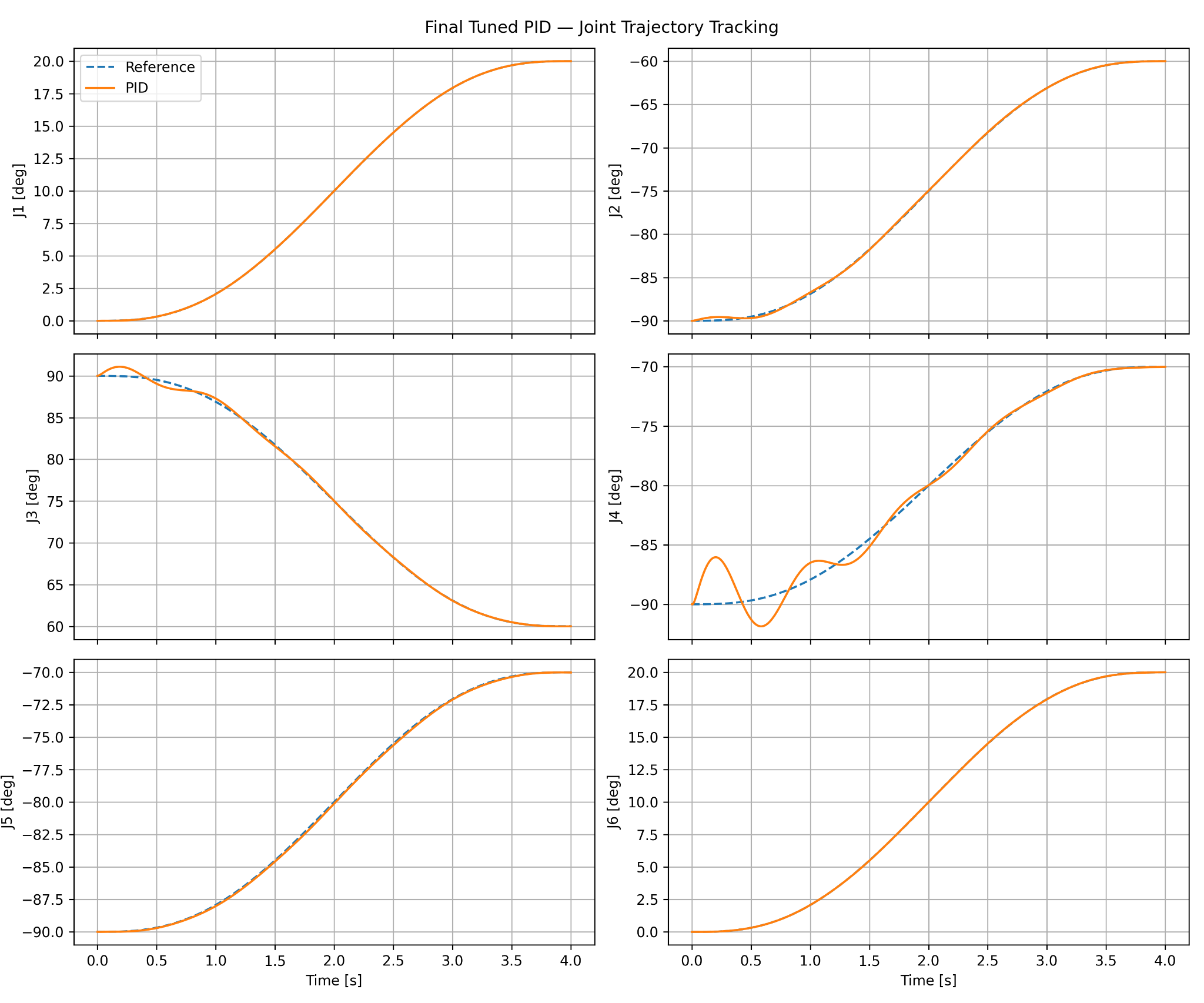
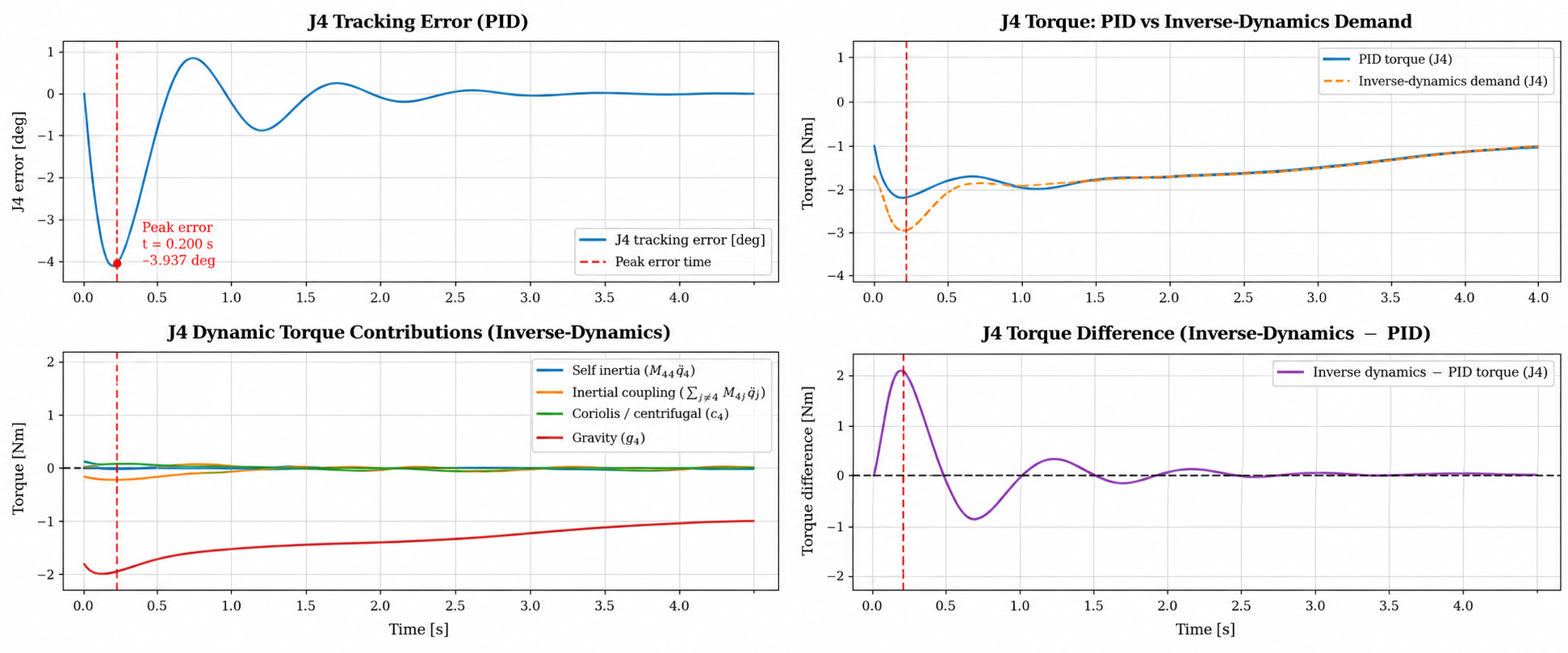
The joint-space PID was tuned through effective-inertia-based bandwidth, damping, and integral-gain studies. The final design uses ωn = 20 rad/s, ζ = 3, and αi = 18. Instead of treating the remaining J4 error as a generic gain problem, I decomposed the dynamics and found that the behavior was primarily gravity dominated rather than saturation or coupling dominated.

**Figure 1 — PID Bandwidth Sweep**Systematic bandwidth study before final damping and integral-action selection.

**Figure 2 — PID Damping Selection**Final damping comparison used to control transient behavior.

**Figure 3 — PID Integral-Gain Selection**Integral action was introduced after the PD structure was established.

**Figure 4 — Final PID Joint Tracking**Common 4 s benchmark tracking with the final PID design.

**Figure 5 — PID Joint Error**Nominal overall joint RMSE: 0.469844°.

**Figure 6 — PID Commanded Torque**The nominal response remains well inside the adopted torque limits.

**Figure 7 — J4 Dynamic Decomposition**The largest PID tracking issue was diagnosed as gravity dominated rather than saturation dominated.

3. Computed Torque — Nominal Accuracy and Model Dependence

Computed-torque control uses the nominal rigid-body model to cancel the modeled dynamics and impose second-order error behavior. With the controller model and plant exactly matched, it achieved 0.001244° overall joint RMSE and 0.004139 mm TCP position RMSE.

τ = M(q)[q̈_d + K_dė + K_pe] + c(q,q̇) + g(q)

The commanded torque closely reproduces the Part 1A inverse-dynamics benchmark. I therefore treated the exceptional nominal result as a reason to test model sensitivity rather than as proof of universal superiority. The 2 kg payload case later exposes that dependence directly.

The measured Python computation time is dominated by the current numerical Coriolis implementation and is not interpreted as an intrinsic timing limit of computed-torque control.

4. Discrete LQR — Diagnosing the Feedforward Structure

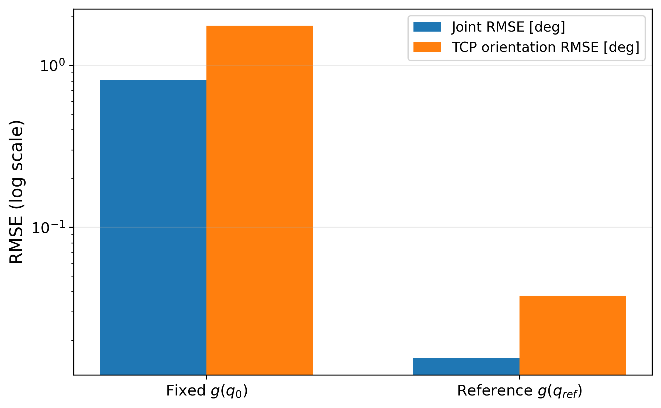
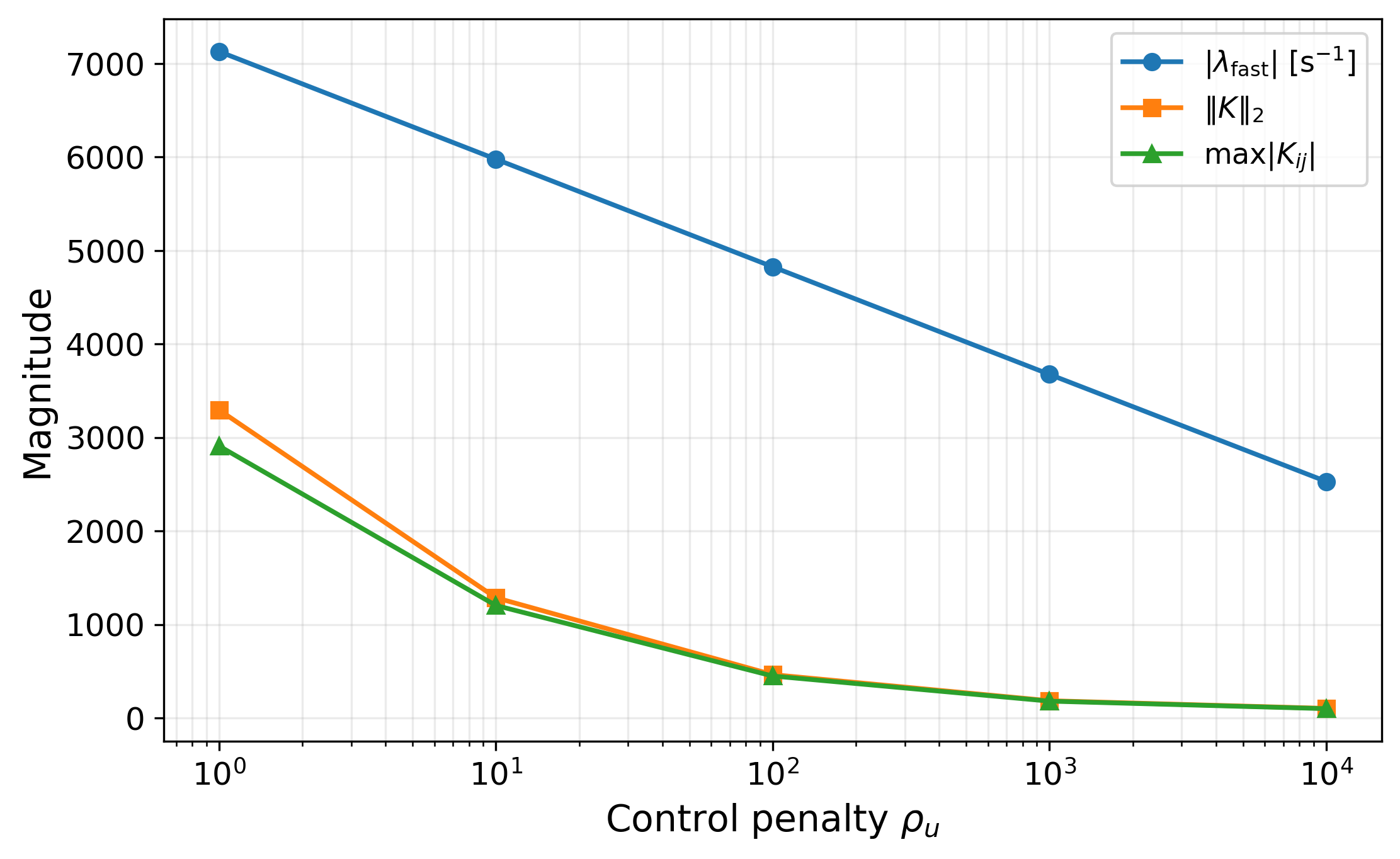
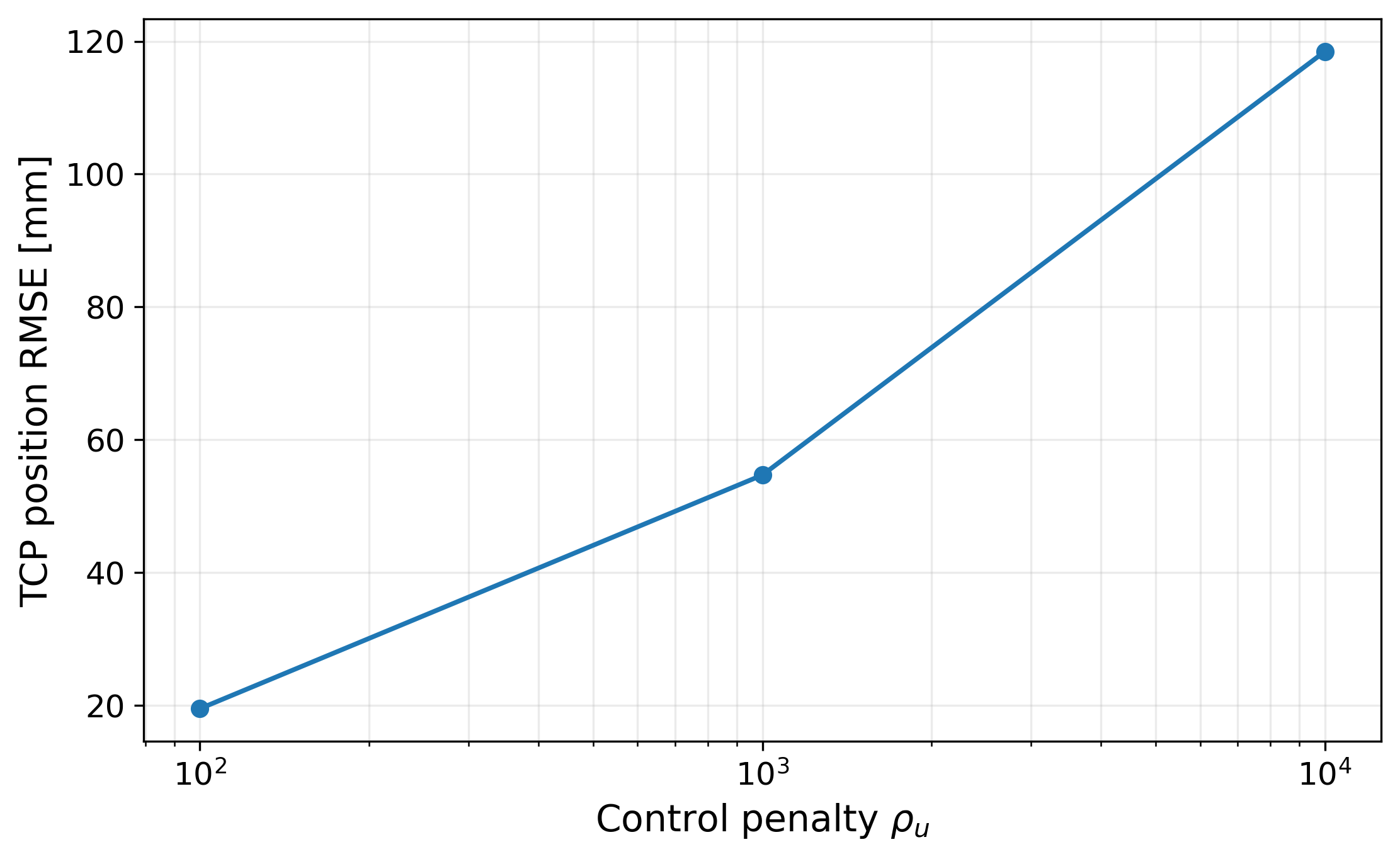
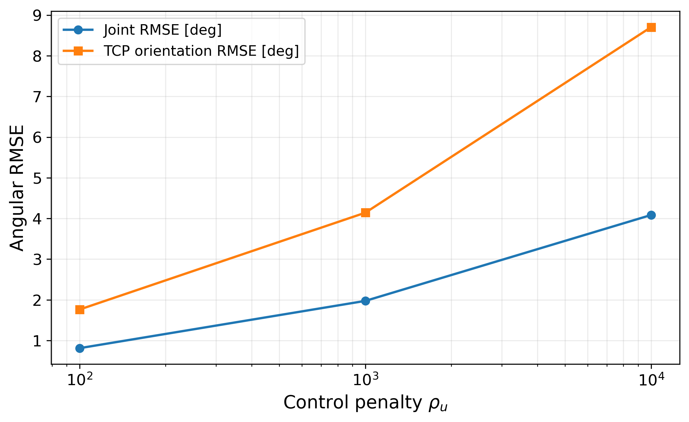
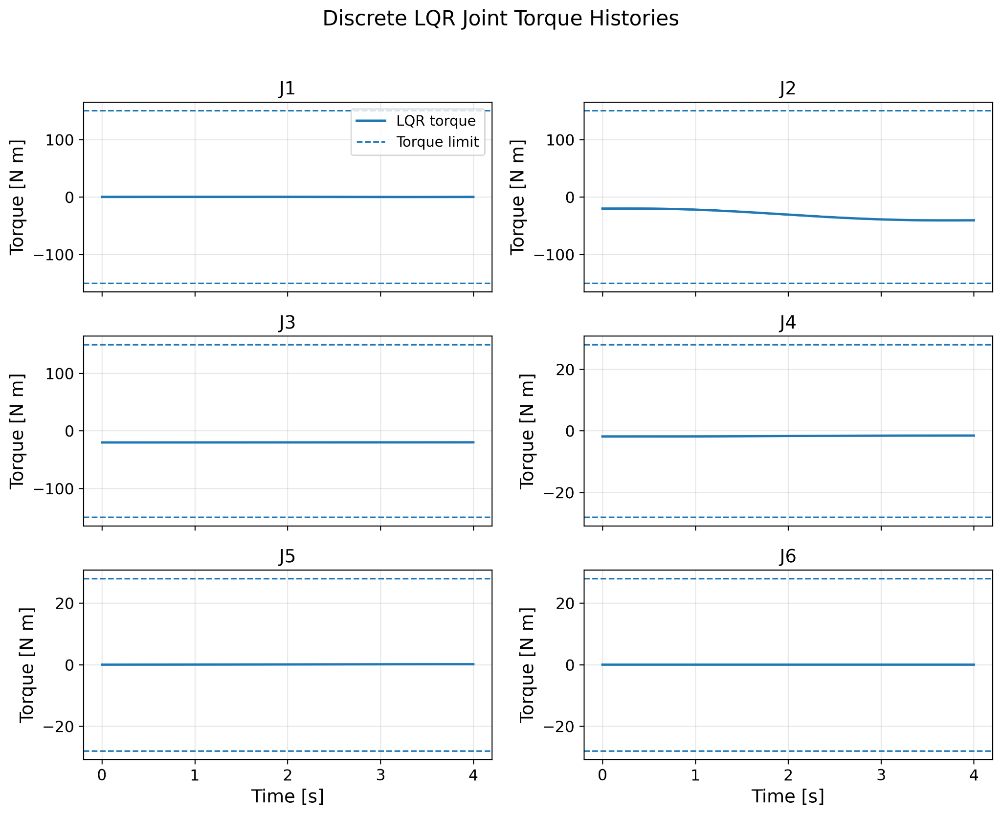
The first local LQR implementation performed poorly on the nonlinear trajectory. The result was retained as a diagnostic step. A fixed equilibrium gravity term did not follow the changing reference configuration. The final design uses exact ZOH discretization, a DARE solution, Bryson-style normalization, ρu = 100, and reference-dependent gravity feedforward.

τ = g(q_ref) − K [ q − q_ref ; q̇ − q̇_ref ]

**Figure 8 — LQR Gravity Feedforward — TCP**Reference-dependent gravity feedforward substantially improved nonlinear trajectory tracking.

**Figure 9 — LQR Gravity Feedforward — Orientation**The result showed that feedforward structure mattered more than repeatedly retuning the same fixed-gravity formulation.

**Figure 10 — LQR Input-Weight Sweep**Gain and closed-loop pole behavior were examined before nonlinear selection.

**Figure 11 — LQR Nonlinear Sweep — TCP**Candidate input penalties were evaluated on the nonlinear plant.

**Figure 12 — LQR Nonlinear Sweep — Orientation**Nonlinear evaluation connected the local design to full-trajectory behavior.

**Figure 13 — Final LQR Joint Tracking**Final overall joint RMSE: 0.015502°.

**Figure 14 — Final LQR Joint Error**Low error was achieved with one fixed nominal linearization plus reference-dependent gravity feedforward.

**Figure 15 — Final LQR Commanded Torque**The common benchmark remains within the modeled torque limits.

5. Constrained MPC — Prediction and Runtime Architecture

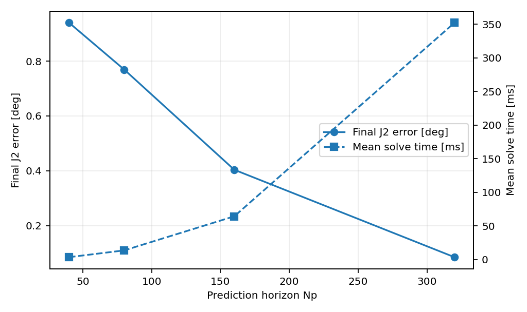
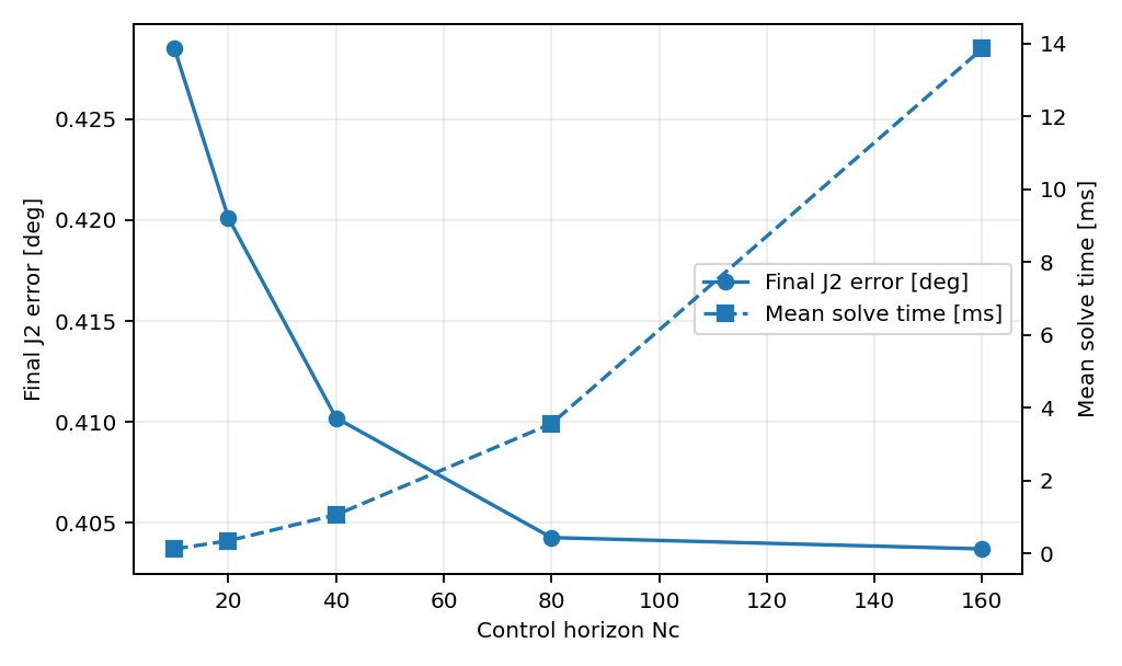
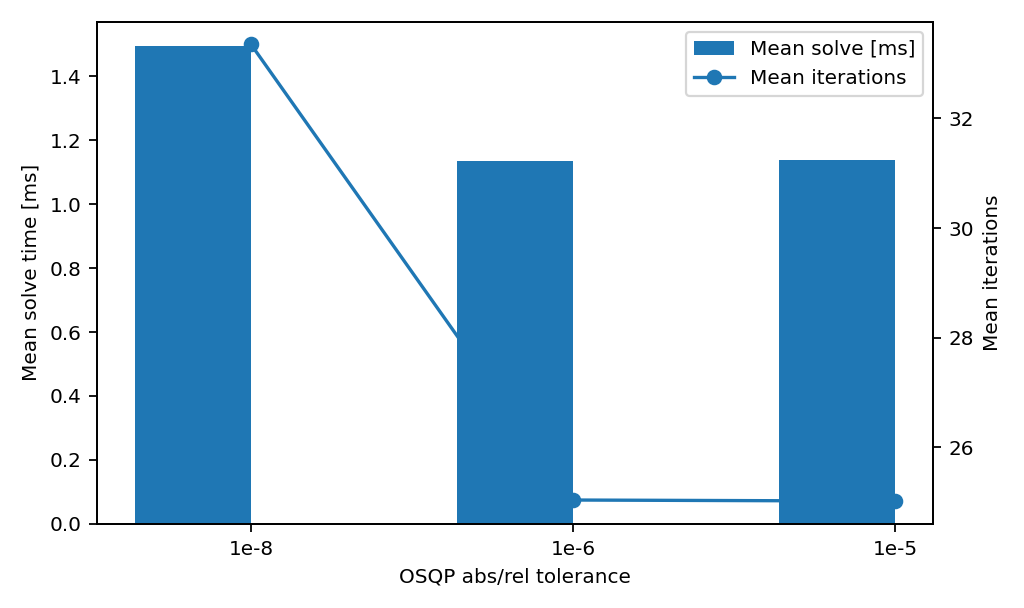
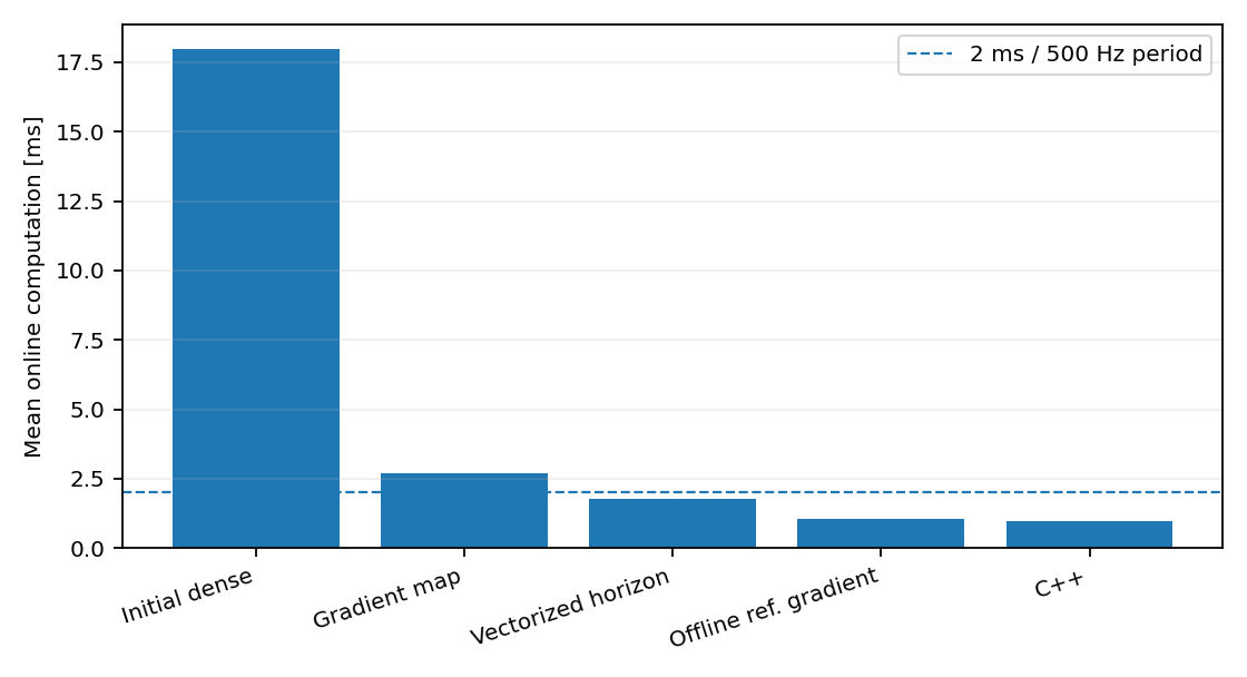
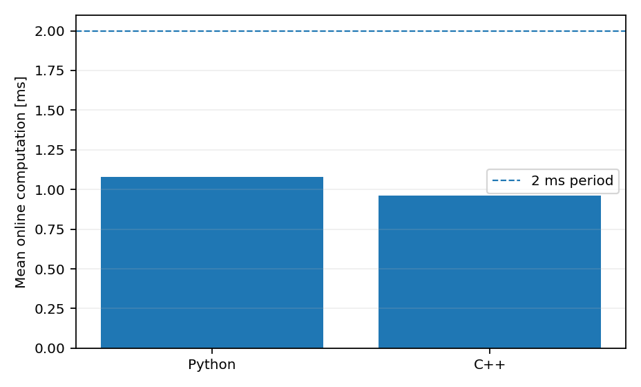
The final linear MPC uses Np = 160 (320 ms), Nc = 40 (80 ms), ρu = 10, and explicit joint-torque constraints in an OSQP quadratic program. Profiling showed that known reference-dependent QP terms were being rebuilt online. I separated the gradient into state-dependent and known reference-dependent components and moved the latter offline, preserving the controller mathematics while reducing online computation.

**Figure 16 — MPC Prediction-Horizon Sweep**Prediction length was selected from measured tracking and computation behavior.

**Figure 17 — MPC Control-Horizon Sweep**A shorter independent control horizon reduces optimization dimension while retaining a longer prediction window.

**Figure 18 — MPC Solver-Tolerance Study**Solver accuracy and computation were evaluated together.

**Figure 19 — MPC Joint Error Metrics**Final overall joint RMSE: 0.048474°.

**Figure 20 — MPC TCP Metrics**Nominal TCP position/orientation RMSE: 0.378424 mm / 0.129772°.

**Figure 21 — MPC Torque Utilization**Constraints are included in the QP, but the nominal benchmark does not activate them.

**Figure 22 — MPC Computation Optimization**Profiling motivated an offline/online algebraic decomposition without changing the controller objective.

**Figure 23 — MPC Python–C++ Timing**C++ mean online time ≈ 0.96 ms with Python–C++ torque agreement ≈ 2 × 10⁻¹⁰ Nm.

6. Robustness Methodology

Nominal accuracy and robustness were intentionally separated. Final controller parameters were frozen and two different perturbation mechanisms were applied to the actual plant.

R1 — Persistent Model Mismatch

A 2.0 kg point payload is placed 0.10 m along tool-frame +Z. The actual plant changes inertia and gravity while every controller continues to use its nominal bare-arm design model.

R2 — External Disturbance

A +20 Nm generalized torque is applied to Joint 2 for 200 ms from t = 2.0 s. The nominal plant itself is unchanged and the controller is not informed of the disturbance.

7. Robustness Results

**Figure 24 — Joint Tracking Robustness**Nominal, 2 kg payload mismatch, and J2 disturbance results.

**Figure 25 — TCP Position Robustness**Cartesian position tracking reveals sensitivity not visible from nominal joint RMSE alone.

**Figure 26 — TCP Orientation Robustness**Persistent model mismatch affects all four controller architectures.

**Figure 27 — Tracking Degradation Relative to Nominal**Relative degradation is interpreted together with absolute error, especially when the nominal denominator is near zero.

**Figure 28 — Control Effort Under Robustness Tests**None of the robustness cases is saturation dominated.

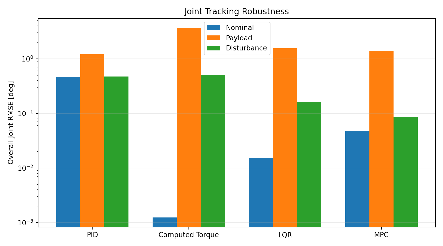
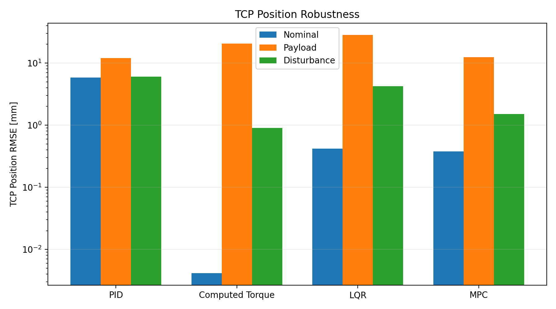
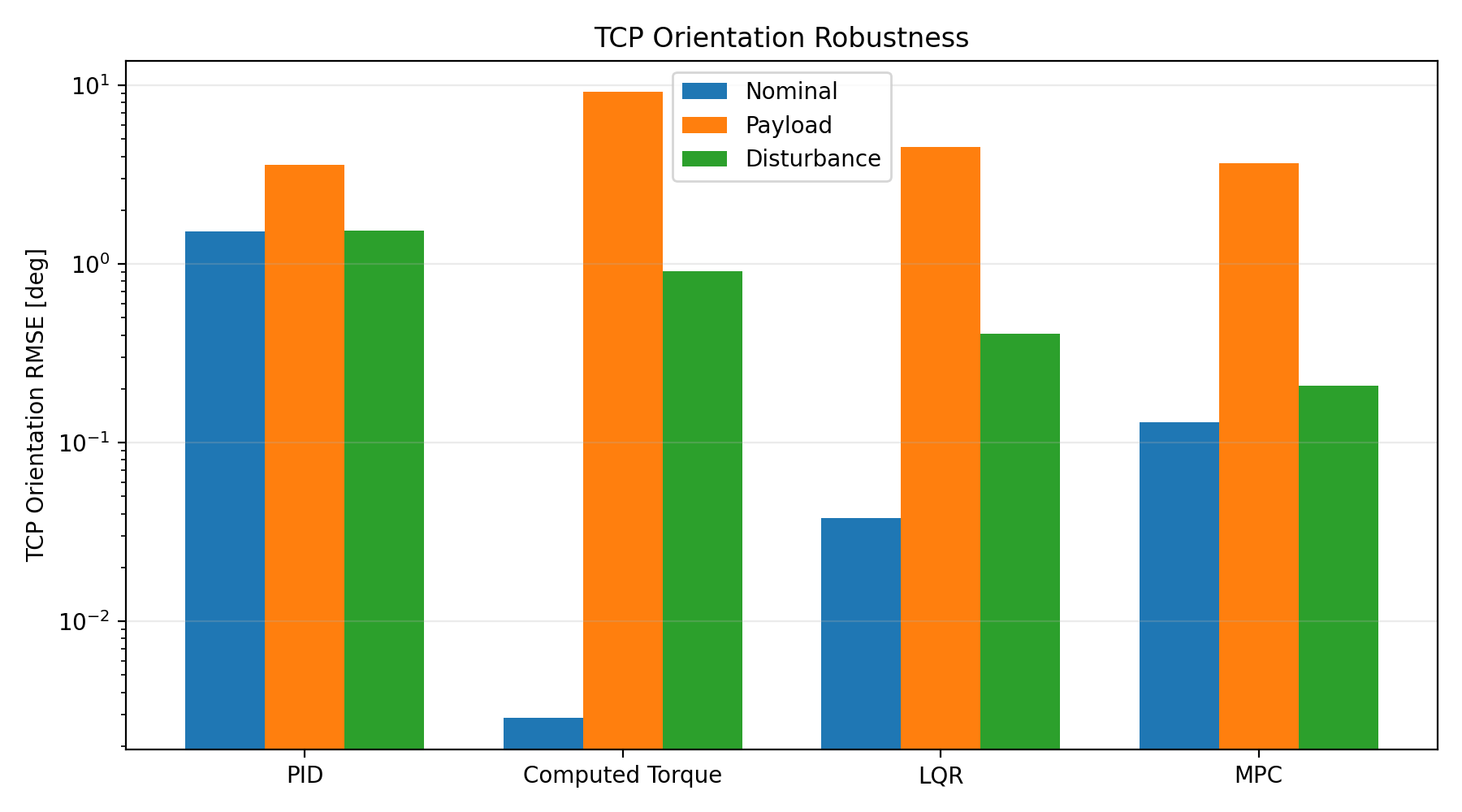
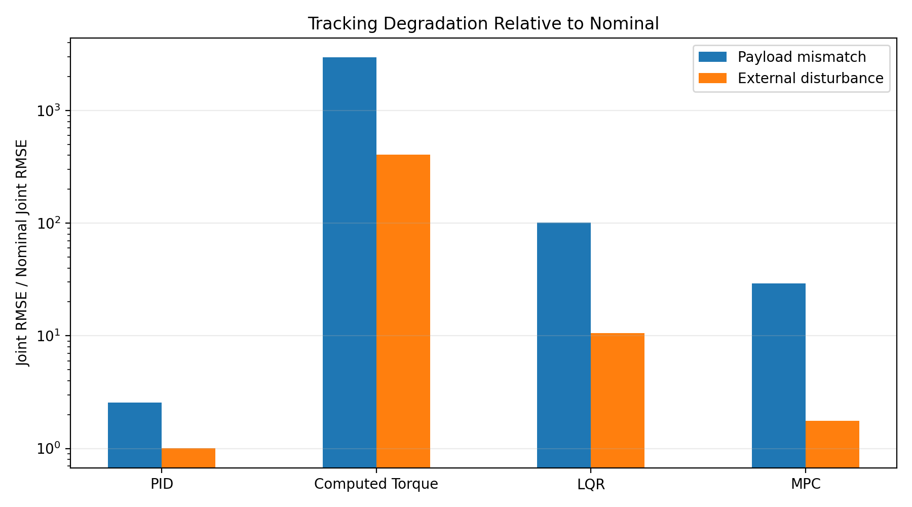
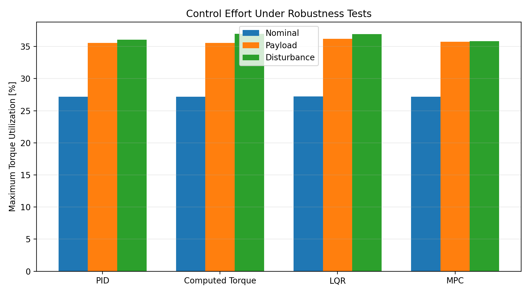
Controller	Case	Joint RMSE [deg]	TCP Position [mm]	TCP Orientation [deg]
PID	Nominal	0.469844	5.835795	1.527910
PID	Payload	1.205309	11.963438	3.585649
PID	Disturbance	0.472416	6.032206	1.531076
Computed Torque	Nominal	0.001244	0.004139	0.002883
Computed Torque	Payload	3.684475	20.562134	9.174375
Computed Torque	Disturbance	0.504513	0.900220	0.907051
LQR	Nominal	0.015502	0.418511	0.037763
LQR	Payload	1.564289	28.293832	4.533704
LQR	Disturbance	0.163066	4.246570	0.406142
MPC	Nominal	0.048474	0.378424	0.129772
MPC	Payload	1.412378	12.380191	3.659589
MPC	Disturbance	0.085670	1.503611	0.209132

8. Engineering Conclusions

Nominal Precision ≠ Robustness

Computed torque is exceptionally accurate under exact model match, while persistent payload mismatch exposes the sensitivity of model cancellation. The two tests measure different properties.

Transient ≠ Persistent Uncertainty

The J2 pulse disappears after 200 ms while the payload mismatch persists. Separating the cases prevents disturbance rejection and model robustness from being treated as the same engineering problem.

Constraints Were Not the Story Here

MPC includes explicit torque constraints, but none of the current tests activates them. The present results therefore support conclusions about tracking, computation, and robustness—not a demonstrated constraint-handling advantage.

Implementation Matters

PID exposed update-order details, LQR exposed feedforward structure, and MPC exposed the distinction between controller mathematics and online software architecture. Python–C++ cross-validation ensured implementation changes preserved the intended controller.

Part 1B conclusion: the useful comparison is not a single controller ranking. PID, computed torque, LQR, and MPC make different assumptions about feedback, model fidelity, prediction, constraints, and computation. Those assumptions become visible only when nominal tracking, model mismatch, disturbance rejection, and implementation behavior are examined together.

9. Technical Reports

Integrated Part 1B Report

Full controller-design, nominal-benchmark, computation, Python–C++ validation, and robustness assessment.

View Full Part 1B Report

PID Controller Report

Detailed tuning, final benchmark, J4 dynamic diagnosis, and implementation analysis.

View PID Report

LQR Controller Report

Discrete design, gravity-feedforward diagnosis, nonlinear tuning, and Python–C++ validation.

View LQR Report

MPC Controller Report

QP formulation, horizon/tolerance studies, computation profiling, offline/online restructuring, and C++ runtime validation.

View MPC Report

← Previous: Part 1A Back to Projects →

Project by Sooyong Kim · Robotics Control Portfolio