Control Systems · Part 1A

UR5e Kinematic & Dynamic Characterization

Starting from the UR5e model established in Pre-Part 1, I characterized the nonlinear plant before controller design. The study examines Jacobian conditioning and singularity approach, pseudoinverse versus damped least-squares behavior, configuration-dependent rigid-body dynamics, equilibrium and local linearization, benchmark feasibility, and Python–C++ numerical consistency.

UR5e Kinematics Jacobian Singularity Rigid-Body Dynamics Linearization C++ / Eigen Control Benchmark

View source on GitHub →

12 / 12 Controllability rank at all three investigated equilibria

1.44 × 10⁻⁹ Maximum skew-symmetry residual in the Coriolis structural test

27.2% Maximum benchmark torque utilization at Joint 2

Engineering objective: characterize the validated plant before controller tuning so that Part 1B compares PID, computed-torque, LQR, and MPC on a common model, trajectory, sampling rate, and actuator constraints.

1. From Model Validation to Plant Characterization

Pre-Part 1 established agreement between the analytical model and Isaac Sim for the physical-link transforms, Jacobian, mass matrix, and gravity generalized forces. Part 1A therefore does not rebuild the model. Instead, it asks which properties of the validated plant matter for controller design: numerical sensitivity near singularity, configuration-dependent inertia and gravity loading, local linear-model validity, controllability, and whether the selected benchmark excites meaningful dynamics without being dominated by saturation.

I retained two compatible representations. Standard DH geometry is used for forward kinematics and the geometric Jacobian, while rigid-body dynamics use the validated URDF physical-link frame chain. CoM locations and inertia tensors remain attached to their physical local link frames rather than being reassigned to DH frames.

2. Kinematic Characterization

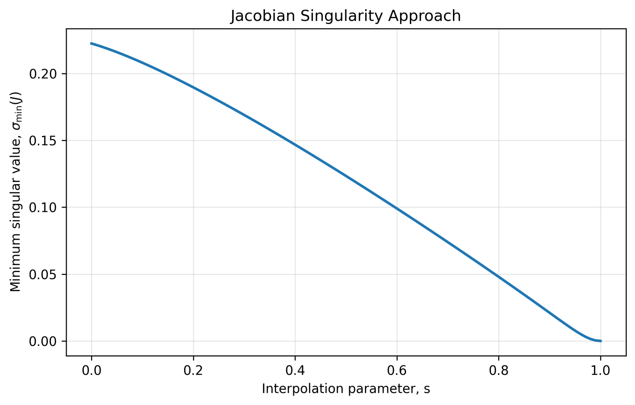
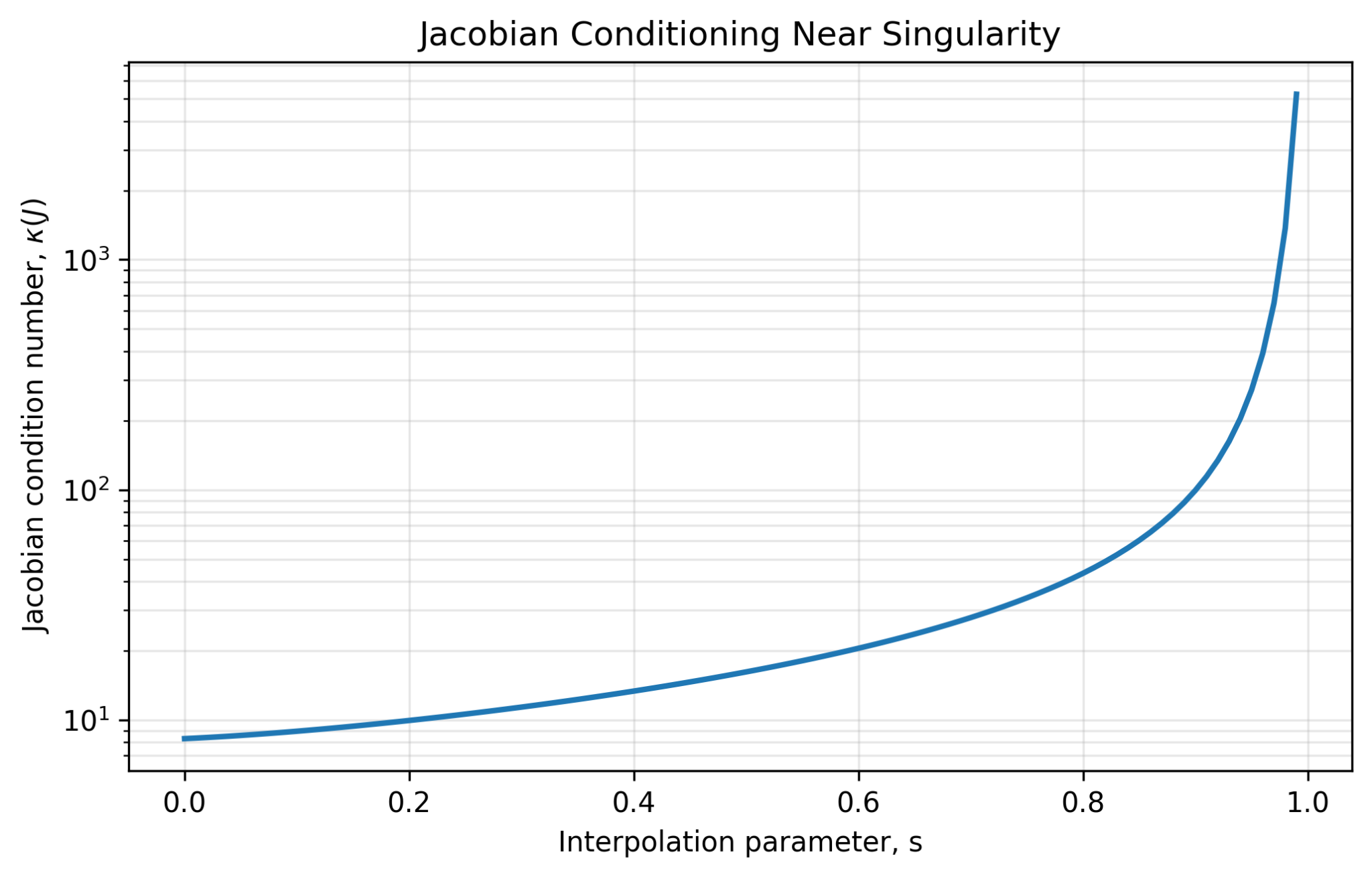
Three configurations were used repeatedly throughout the analysis: the validated test pose [10, -40, 60, -30, 45, 20]°, the nominal working pose [0, -90, 90, -90, -90, 0]°, and the zero configuration. The nominal pose remained well conditioned, whereas the zero configuration lost one instantaneous rotational degree of freedom and reduced the full geometric Jacobian rank to five.

Configuration	σmin(J)	κ(J)	Rank
Validated test pose	0.15682	12.95	6
Nominal working pose	0.22236	8.31	6
Zero configuration	≈ 0	∞	5

3. Singularity Approach: Conditioning Before Rank Loss

I interpolated from the nominal working pose to the zero configuration. The minimum singular value decreased continuously toward zero while the condition number increased sharply before exact rank loss. This is important for control and inverse kinematics: a matrix can remain formally full rank while already becoming numerically aggressive.

Minimum singular value along the UR5e nominal-to-singular sweep — **Figure 1 — Minimum Singular Value Near Singularity** The minimum singular value decreases continuously as the trajectory approaches the zero configuration, exposing the loss of numerical robustness before exact rank loss.

UR5e Jacobian condition number near singularity — **Figure 2 — Jacobian Condition Number** The condition number rises rapidly on the approach to the singular configuration, demonstrating why a binary rank test alone is insufficient for numerical robustness.

4. Pseudoinverse vs. Damped Least Squares

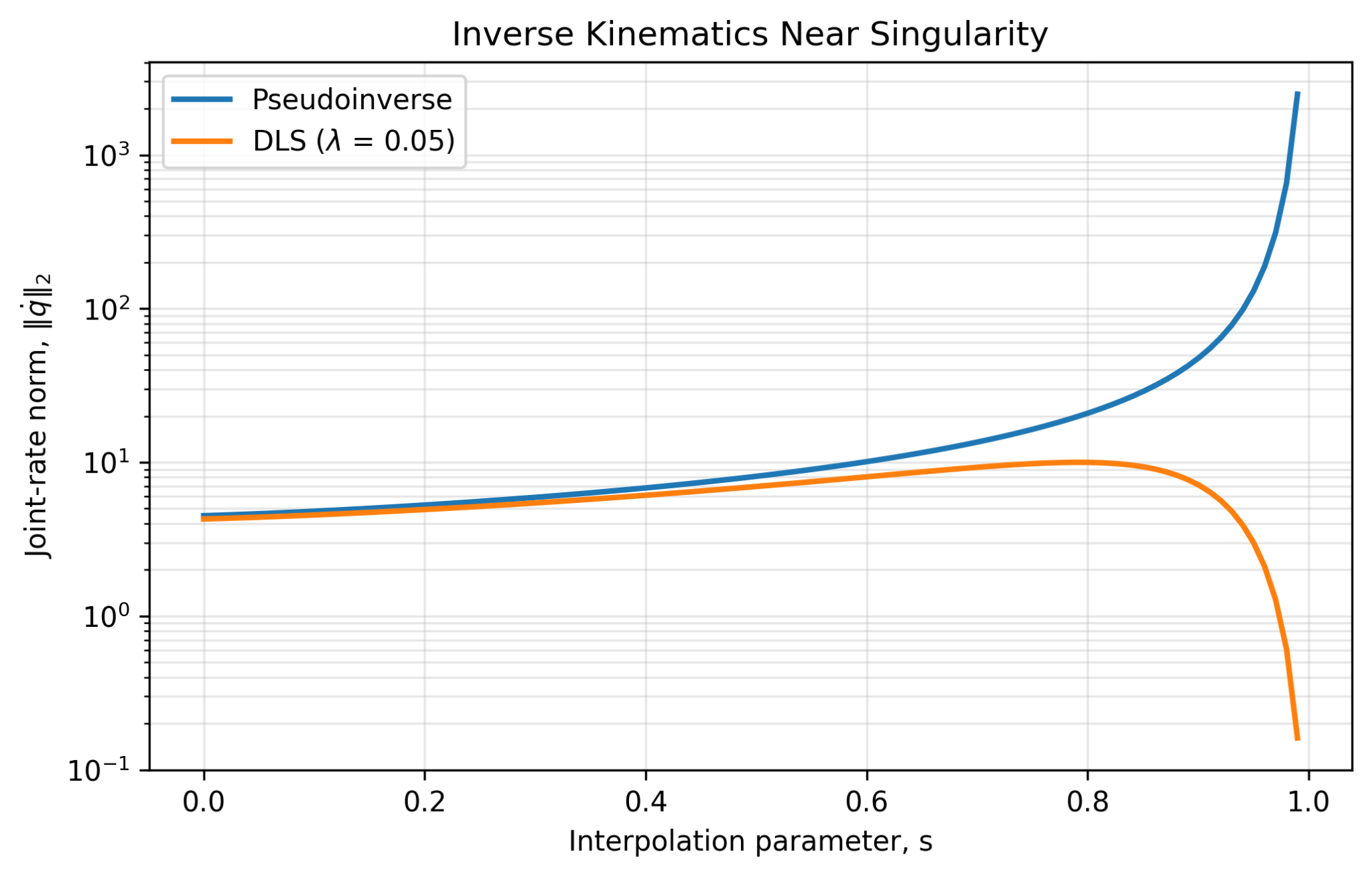
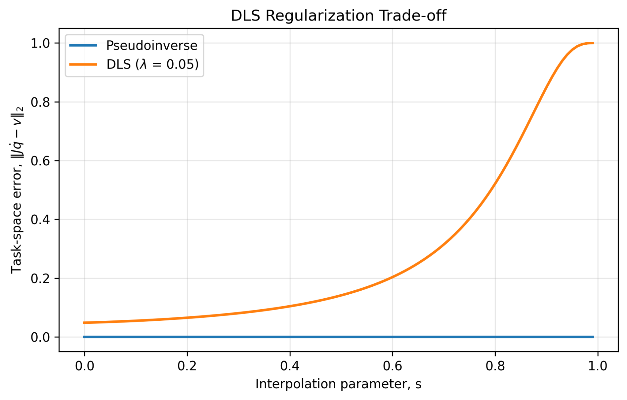
To expose the weakest instantaneous task direction, I commanded a unit task-space velocity along the weakest left-singular vector. The Moore–Penrose pseudoinverse preserved the command but produced rapidly increasing joint-rate demand. Damped least squares (DLS), with λ = 0.05, bounded the amplification by deliberately accepting task-space error.

G_DLS(σ) = σ / (σ² + λ²), G_DLS,max = 1 / (2λ) = 10

Because the commanded task velocity is a unit vector in the weakest singular direction, the plotted DLS joint-rate norm directly follows this scalar gain. The sweep is discrete, so it need not sample exactly σ = λ; an observed peak slightly below the theoretical maximum of 10 is therefore expected.

Pseudoinverse and damped least squares joint rate comparison — **Figure 3 — Joint-Rate Amplification** The pseudoinverse becomes increasingly aggressive near singularity, while DLS bounds the amplification and then suppresses the weakest direction.

Damped least squares task-space error near singularity — **Figure 4 — DLS Robustness–Accuracy Trade-Off** Bounded joint-rate amplification is obtained by accepting increasing task-space error as the singular direction becomes poorly controllable.

5. Configuration-Dependent Rigid-Body Dynamics

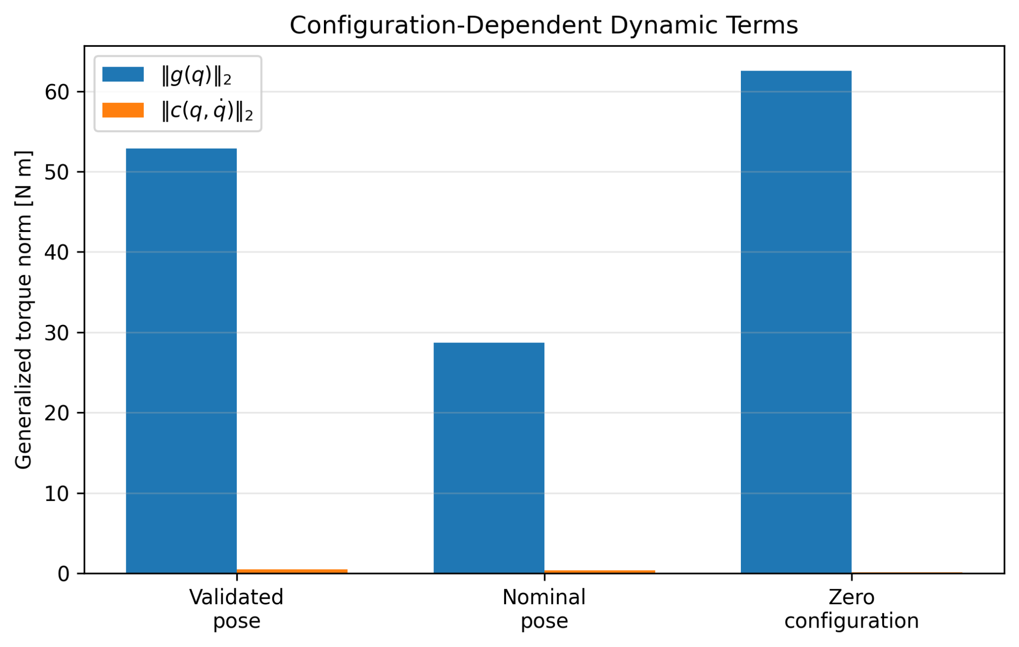
The mass matrix remained symmetric positive definite at all three investigated poses, but its eigenvalue spread, gravity loading, and Coriolis/centrifugal contribution changed substantially with configuration. The large mass-matrix condition numbers are not interpreted as dynamic instability; they reflect anisotropic generalized inertia and motivate solving the dynamics as a linear system rather than explicitly forming M(q)⁻¹.

Configuration	κ(M)	\|\|g\|\| [Nm]	\|\|c\|\| [Nm]
Validated test pose	15101	52.862	0.5303
Nominal working pose	11713	28.716	0.4021
Zero configuration	18587	62.537	0.1581

Configuration dependent gravity and Coriolis torque norms — **Figure 5 — Configuration-Dependent Dynamics** Gravity and Coriolis/centrifugal generalized-torque norms at the three representative configurations for the specified test velocity.

6. Coriolis Structural Consistency

The Coriolis/centrifugal implementation was first checked using c(q,0) = 0 and the expected quadratic velocity dependence c(q,2q̇) = 4c(q,q̇). I then explicitly constructed the Christoffel-based matrix C(q,q̇) and tested both its agreement with the existing vector implementation and the standard rigid-body structural identity.

c(q,q̇) = C(q,q̇)q̇

R = (Ṁ − 2C) + (Ṁ − 2C)^T

Validation Quantity	Maximum Residual
max \|Cq̇ − c\|	8.33 × 10⁻¹⁷
max \|(Ṁ − 2C) + (Ṁ − 2C)^T\|	1.44 × 10⁻⁹

These results provide strong internal structural-consistency evidence for the numerical Christoffel implementation. They are intentionally described as internal model checks, not as an independent physics-engine validation.

7. Nonlinear Plant, Equilibria, and Linearization

The controller plant is a 12-state nonlinear torque-driven system. Static equilibria were defined with zero joint velocity and gravity-compensation input. Numerical linearization about the validated, nominal, and zero configurations produced full controllability rank 12/12 in all three cases.

ẋ = [ q̇ ; M(q)⁻¹(τ − c(q,q̇) − g(q)) ]

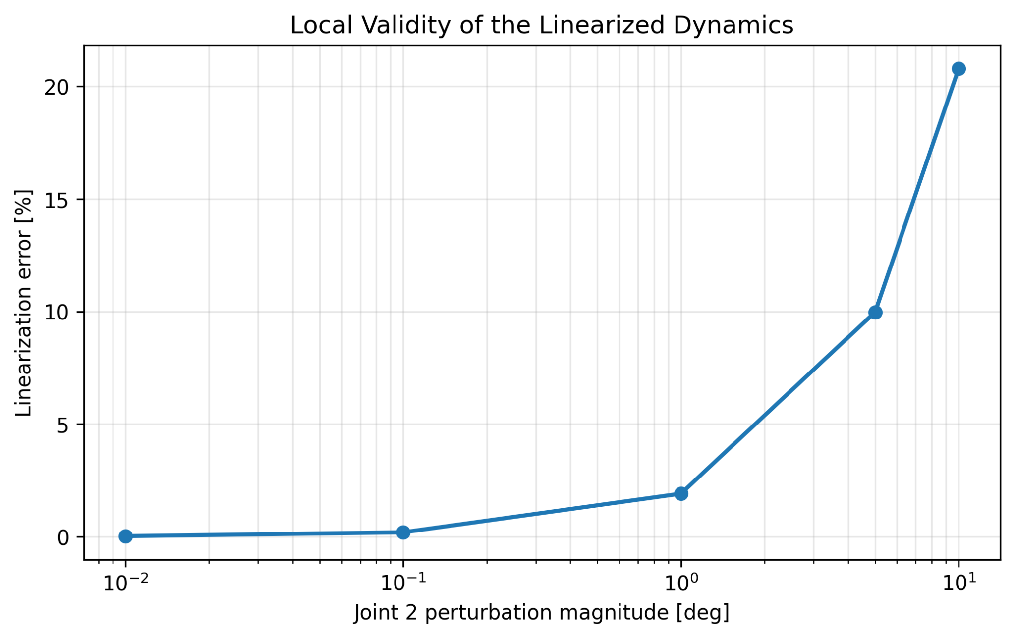
To quantify how local the nominal linear model actually is, I perturbed Joint 2 while holding the equilibrium torque fixed. Relative linearization error increased from 0.0188% at 0.01° to 1.91% at 1°, 9.97% at 5°, and 20.79% at 10°. This gives a measured basis for interpreting the later LQR results rather than assuming one linearization represents the entire motion.

UR5e local linearization validity error — **Figure 6 — Local Linearization Validity** Relative error grows systematically with Joint-2 perturbation magnitude around the nominal equilibrium, demonstrating the local nature of the linear plant model.

8. Common Controller Benchmark

Before tuning any controller, I fixed one common trajectory and one set of simulation constraints. The benchmark moves from [0, -90, 90, -90, -90, 0]° to [20, -60, 60, -70, -70, 20]° in 4.0 s using quintic time scaling, sampled at 2 ms.

h(s) = 10s³ − 15s⁴ + 6s⁵

Common UR5e quintic controller benchmark trajectory — **Figure 7 — Common Joint-Space Benchmark** The 4 s quintic trajectory provides identical reference position, velocity, and acceleration profiles for every Part 1B controller.

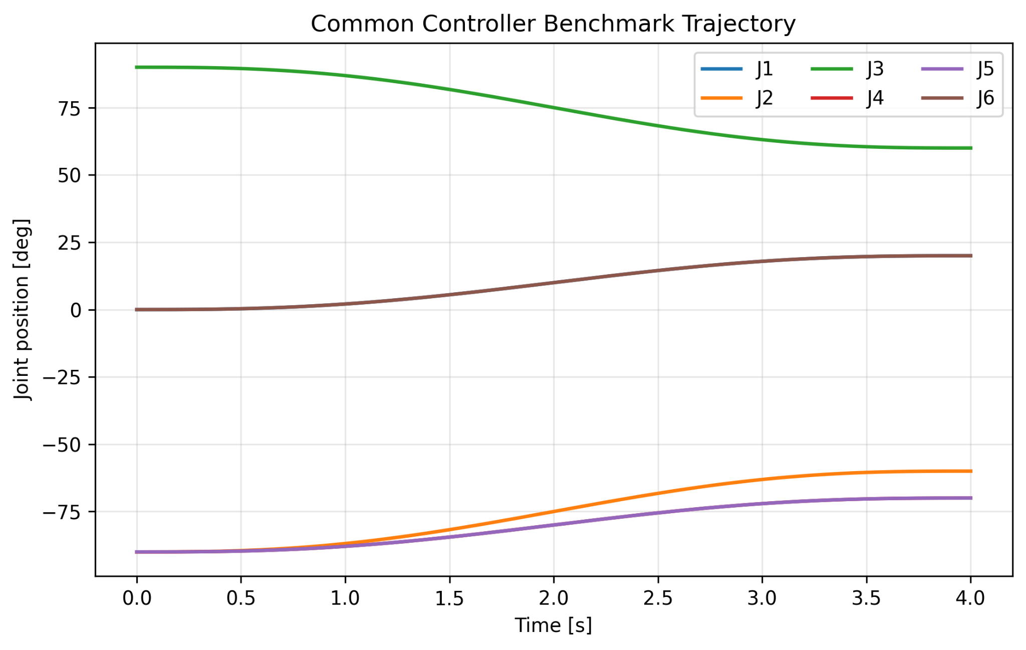
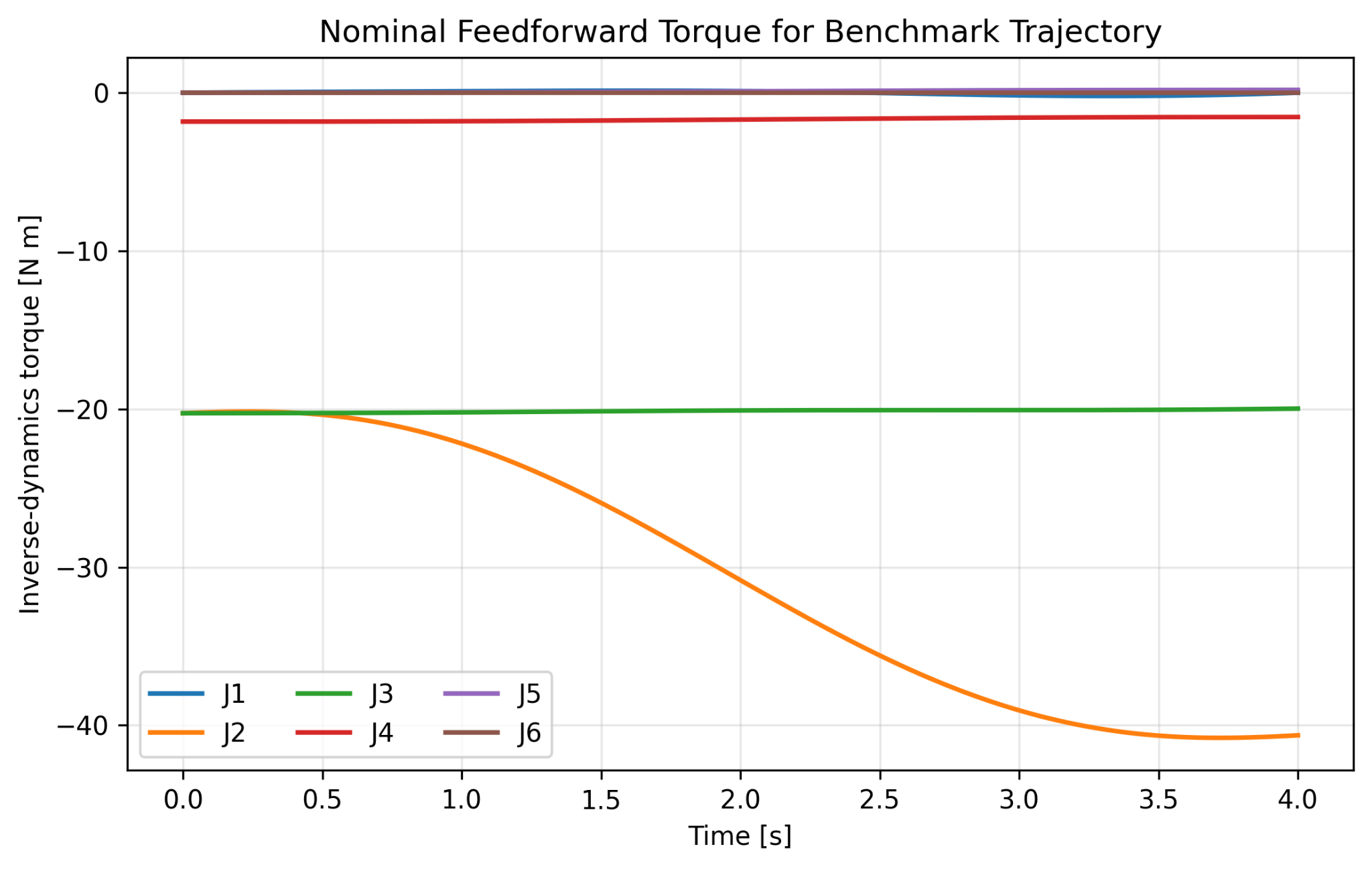
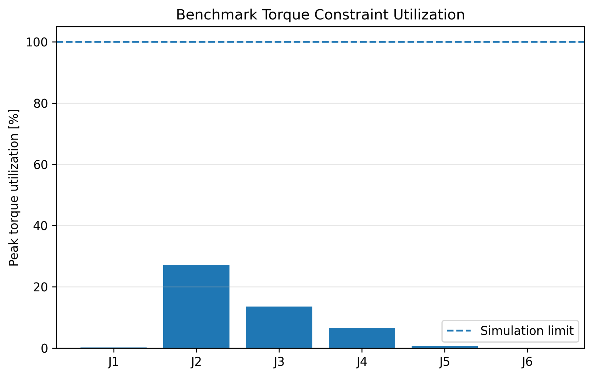
The maximum reference velocity is only 7.81% of the 180°/s joint-speed specification. Nominal inverse dynamics also remain comfortably inside the adopted simulation torque constraints, so the benchmark is dynamically meaningful without being primarily a saturation test.

UR5e inverse dynamics feedforward torque over the benchmark trajectory — **Figure 8 — Nominal Inverse-Dynamics Torque** Feedforward torque along the common benchmark, including inertial, Coriolis/centrifugal, and gravity contributions.

UR5e benchmark torque utilization by joint — **Figure 9 — Benchmark Torque Utilization** Joint 2 is the most demanding axis at 27.2% of the adopted simulation torque constraint; all six joints remain within the common limits.

9. Python–C++ Cross-Validation

Python remains the numerical reference environment for analysis, plotting, parameter studies, and controller tuning. I reproduced the core plant in fixed-size C++/Eigen for later runtime controller work. The C++ dynamics intentionally use the same validated physical-link formulation rather than attaching inertia data directly to the DH chain.

Quantity	Maximum Error	Result
TCP position	3.80 × 10⁻⁹	PASS
Jacobian singular values	2.51 × 10⁻⁹	PASS
Mass matrix M(q)	4.93 × 10⁻¹⁰	PASS
Gravity vector g(q)	2.63 × 10⁻⁸	PASS
Coriolis vector c(q,q̇)	5.60 × 10⁻¹⁰	PASS
Trajectory midpoint / endpoints	0 at reported precision	PASS

Python–C++ agreement is an implementation-consistency check, not an independent physics-engine validation. The independent analytical–Isaac comparison was completed in Pre-Part 1.

10. Engineering Conclusions

What Part 1A Established

Singularity sensitivity appears before rank loss, rigid-body dynamics change materially with configuration, the nominal linear model is demonstrably local, and the selected benchmark is feasible without being saturation dominated.

What Part 1B Must Test

PID, computed-torque, LQR, and MPC can now be compared on identical plant, trajectory, sampling, and constraint assumptions, with explicit attention to configuration dependence, model mismatch, control effort, and computation.

11. Technical Report

Part 1A Technical Report

The full report documents the mathematical formulation, numerical characterization, structural consistency tests, local linearization study, benchmark definition, Python–C++ cross-validation, limitations, and reproducibility map in greater detail.

View Technical Report

← Previous: Model Validation Back to Projects →

Project by Sooyong Kim · Robotics Control Portfolio