Modeling & Control · Reinforcement Learning

Model-Based and Learning-Based Control of a 2-DOF Manipulator

This project asks a practical control question: when the analytical model is imperfect, is it better to replace the controller with model-free reinforcement learning, or to preserve the known physics and learn only the missing dynamics? The study connects controlled model mismatch to actuator-level torque deficit, then compares exact-model CTC, mismatched CTC, Pure SAC, and CTC + Residual SAC on the same Cartesian end-effector task.

Computed Torque Control Soft Actor-Critic Residual RL 2-DOF Manipulator Cartesian Tracking Model Mismatch Torque-Deficit Analysis

View source on GitHub →

0.195 mmExact-model CTC Stage-3 end-effector RMSE

31.116 mmCTC RMSE after a 30% link-2 mass underestimate

4.662 mmFinal Pure SAC Stage-3 RMSE

1.290 mmFinal Residual SAC Stage-3 RMSE

Engineering objective: the goal is not to prove that reinforcement learning is universally superior to classical control. The study first establishes how well model-based control performs when its assumptions are correct, deliberately breaks one of those assumptions, identifies the missing physical torque, and then tests two learning strategies against that failure mode.

1. Study Design

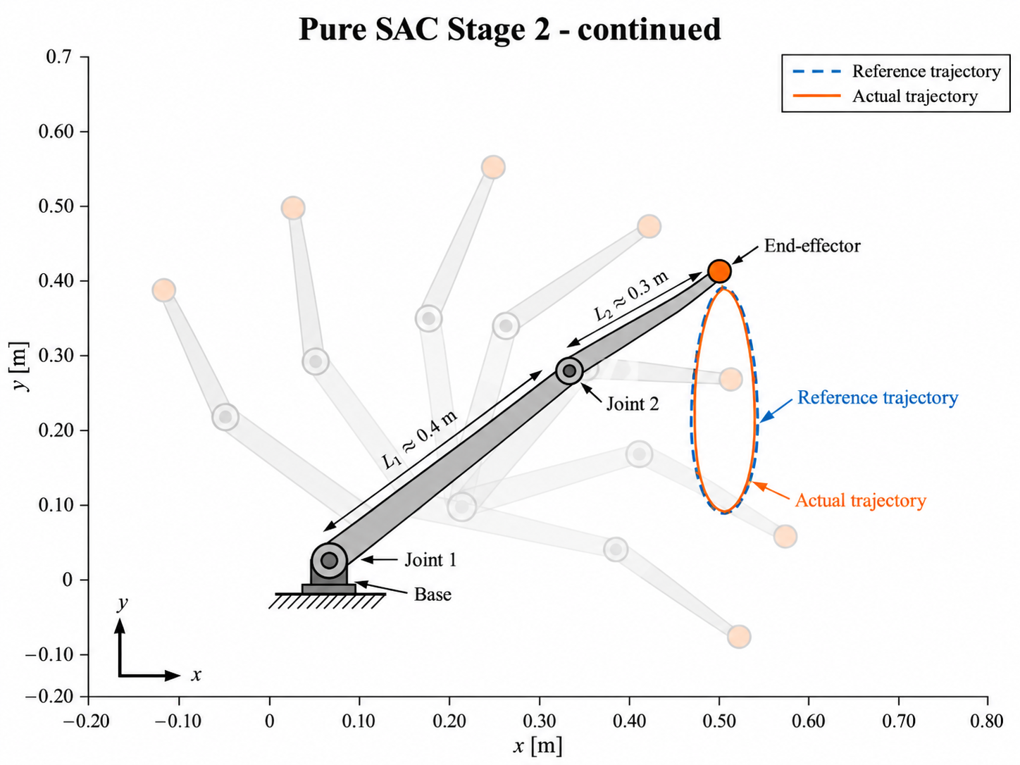
A 2-DOF planar manipulator is used because it is the minimum system that still preserves the nonlinear effects needed for a meaningful control study: configuration-dependent inertia, gravity, Coriolis and centrifugal terms, multi-joint coupling, forward/inverse kinematics, and the distinction between joint-space and Cartesian task-space behavior. The final task is end-effector trajectory tracking; joint references are internal quantities used where required by the model-based controller.

Exact-Model CTCEstablish the ideal model-based reference

Model MismatchIntroduce one traceable physical error

Torque DeficitIdentify what the wrong model is missing

Pure SACLearn the full actuator command

Residual SACLearn only the missing correction

Learning-control system schematic — **Figure 1 — Control Architectures**The same nonlinear plant and Cartesian tracking task are used to compare model-based, model-free, and residual learning architectures.

2. Exact Model vs. Structured Model Error

With the controller model matched to the plant, computed-torque control provides a very strong nominal reference: Stage-3 Cartesian RMSE is only 0.195 mm. This result is treated as an ideal model-consistency benchmark, not a prediction of hardware accuracy.

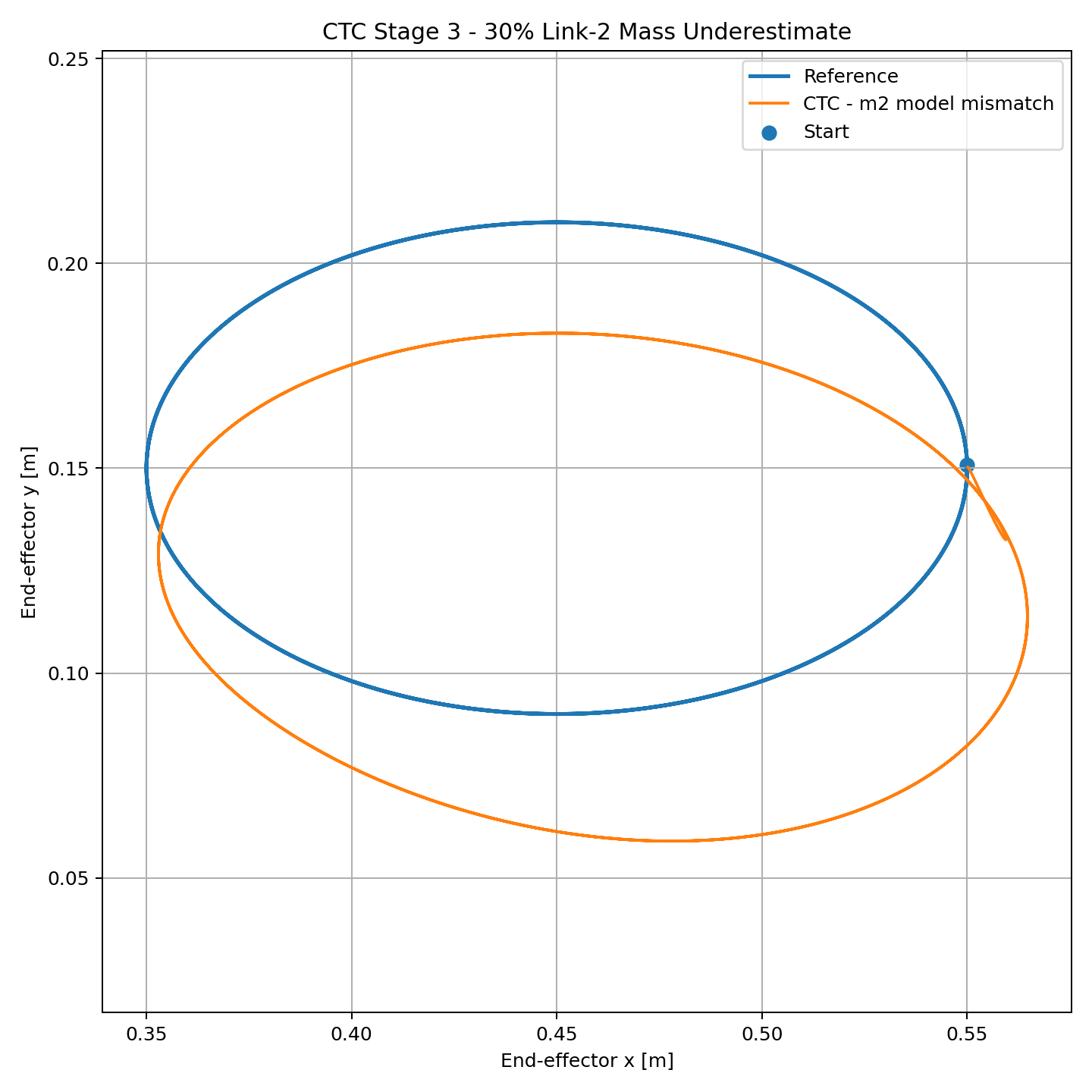
The robustness study then changes only the controller's estimate of the second-link mass, from the true 1.50 kg to 1.05 kg—a 30% underestimate. Keeping every other parameter unchanged makes the degradation physically traceable instead of hiding it inside broad randomization.

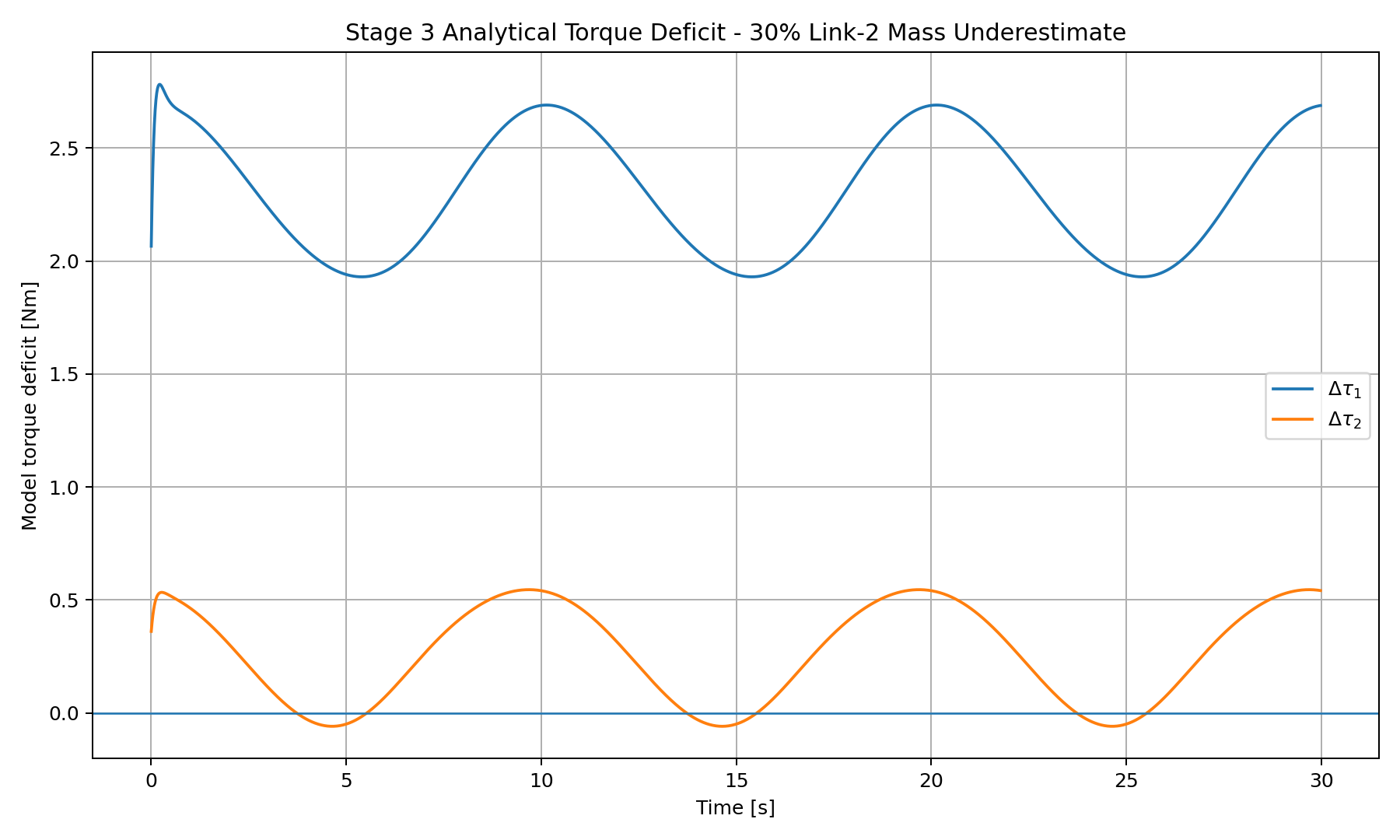
CTC trajectory under 30 percent link-2 mass mismatch — **Figure 2 — CTC Under 30% Link-2 Mass Underestimate**The controller remains unsaturated, but the wrong dynamics compensation produces a systematic task-space bias and raises RMSE to 31.116 mm.

Δτ_model = τ_{true model} − τ_{wrong model}

Rather than stopping at the observation that the trajectory is wrong, the study computes the torque missing from the mismatched controller at the same state and reference. The dominant deficit appears at joint 1, where the closed-loop mismatch trajectory shows approximately 2.318 Nm RMS missing torque.

Analytical model torque deficit under the link-2 mass mismatch — **Figure 3 — Analytical Model Torque Deficit**The model error is converted into an actuator-level quantity that can later be compared directly with the learned residual torque.

3. Pure SAC — Learning the Full Control Law

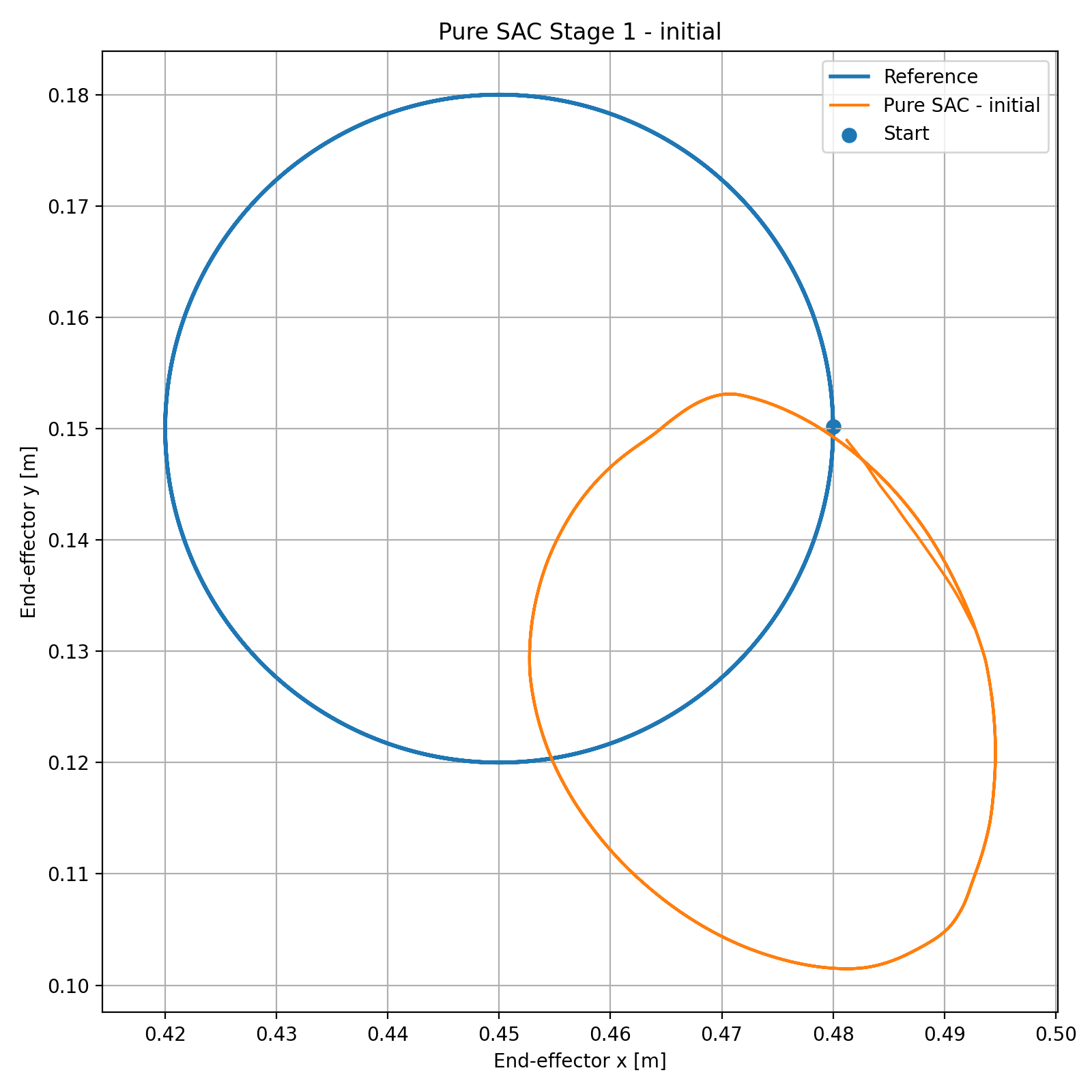
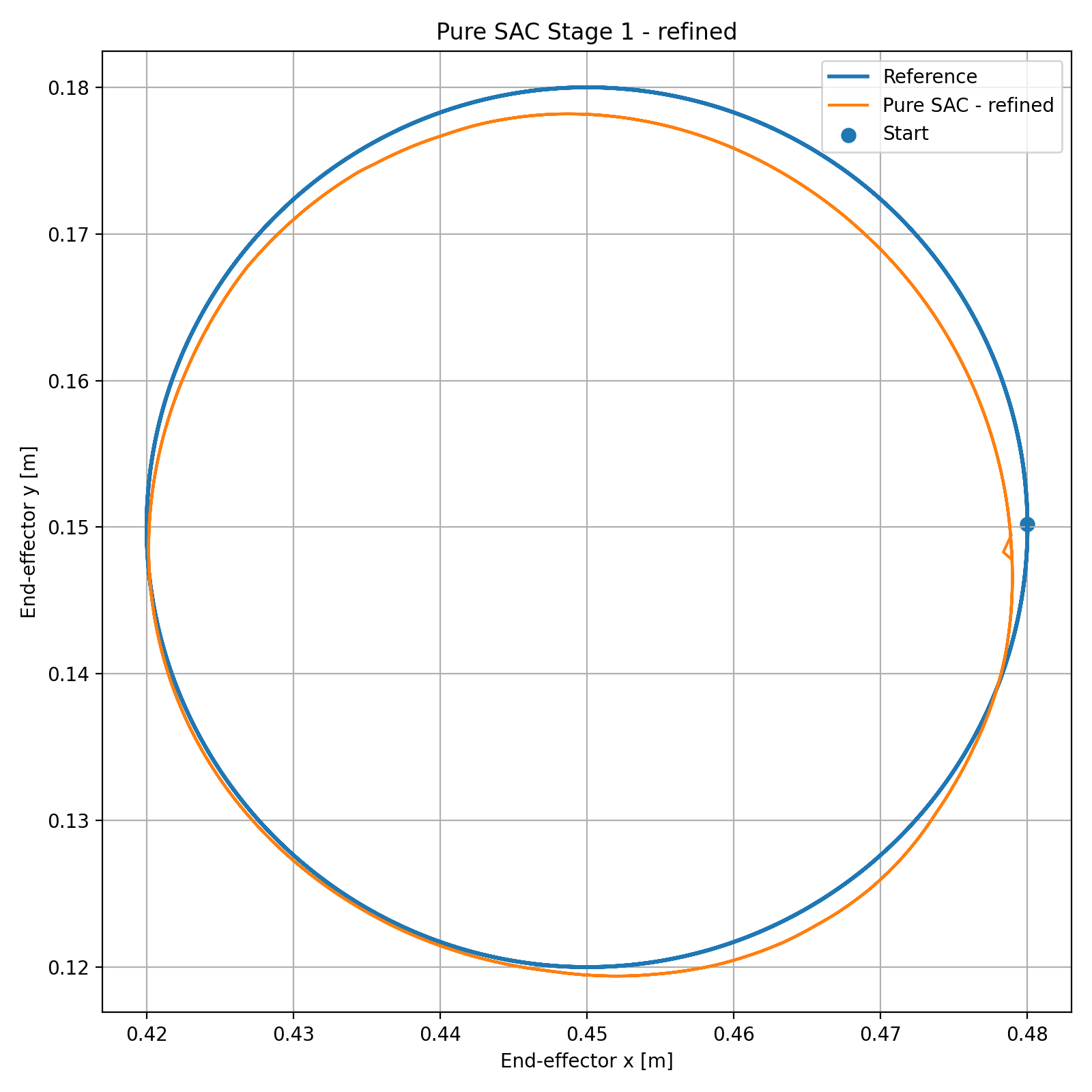
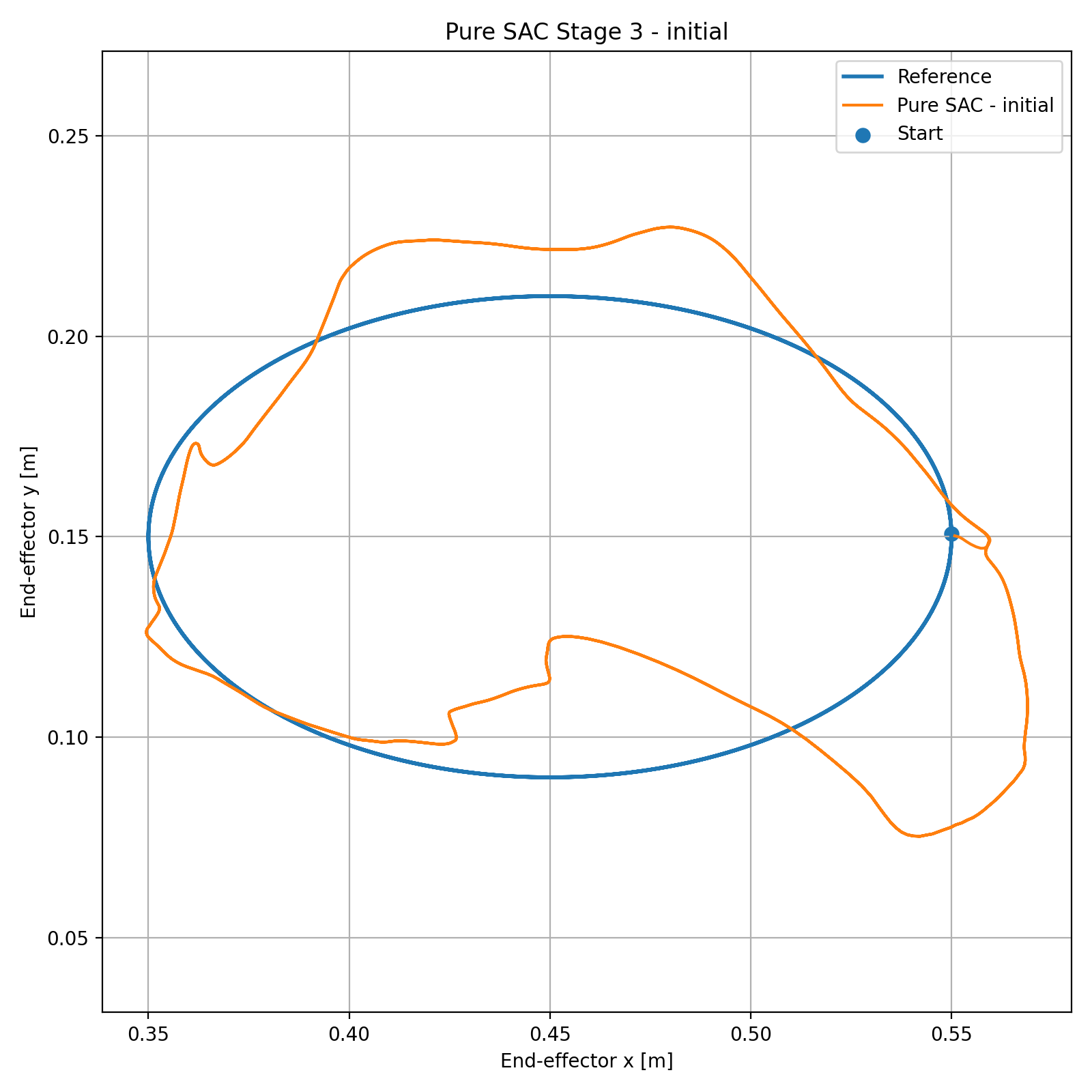
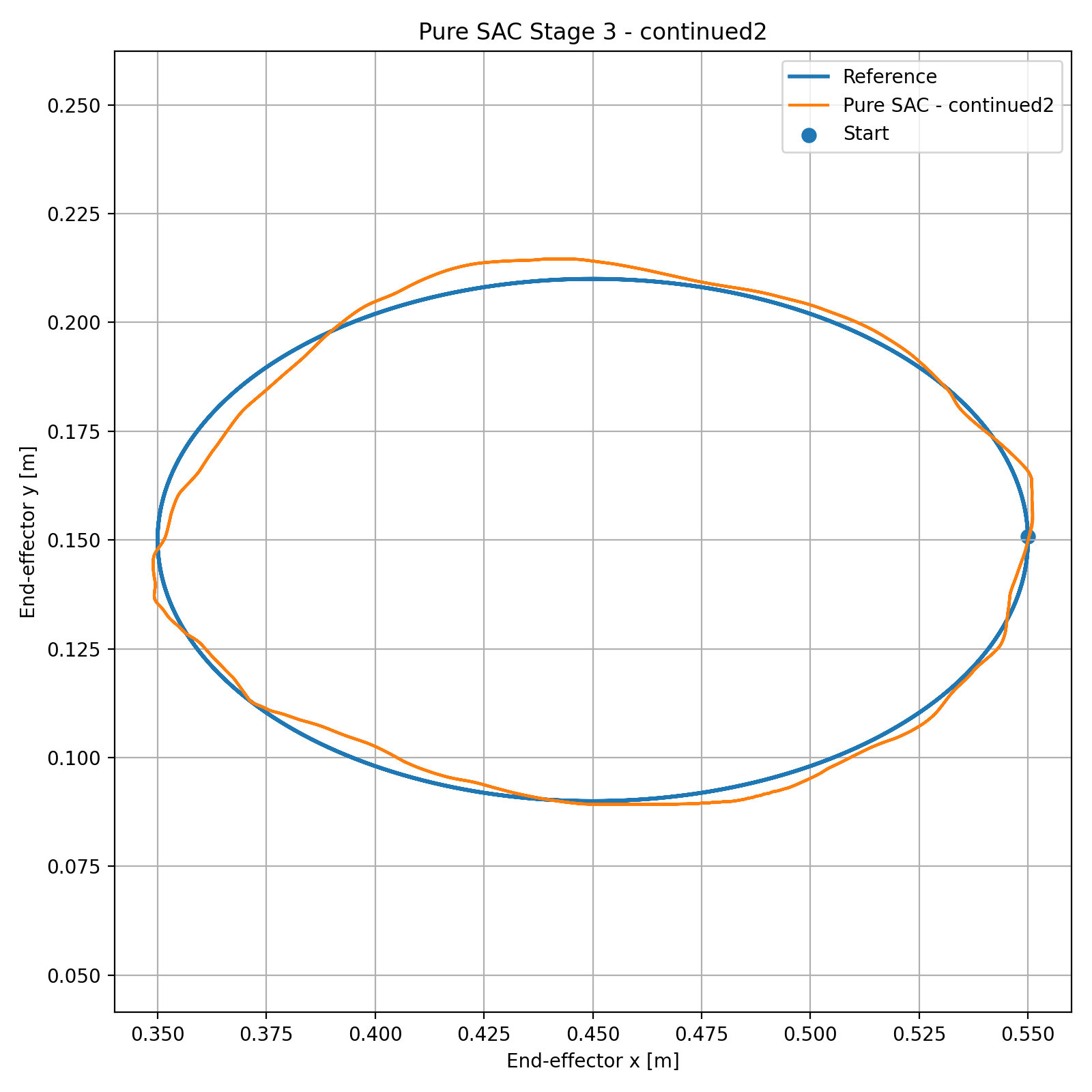
Pure SAC receives the robot state and Cartesian reference and directly generates normalized actuator commands over the full physical torque range. No analytical inverse-dynamics terms are exposed to the policy. Because the final Stage-3 task combines geometry, phase, joint coordination, and higher velocity/acceleration demand, training progresses through a Cartesian curriculum rather than starting from the hardest trajectory.

Pure SAC Stage 1 initial trajectory — **Figure 4 — Pure SAC Stage 1, Initial Training**The initial model-free policy has not yet learned the basic Cartesian circle and shows large geometric distortion.

Pure SAC Stage 1 refined trajectory — **Figure 5 — Pure SAC Stage 1, Refined**After refinement, the same policy architecture reproduces the simple reference closely enough to transfer the learned control structure to harder stages.

Pure SAC Stage 3 initial trajectory — **Figure 6 — Pure SAC Stage 3, Initial Transfer**The harder Stage-3 ellipse initially exposes substantial residual error despite earlier curriculum learning.

Pure SAC Stage 3 final trajectory — **Figure 7 — Pure SAC Stage 3, Final**After continued training, Pure SAC reaches 4.662 mm Cartesian RMSE and 93.994% geometric IoU.

Pure SAC finding: the model-free controller avoids explicit dependence on the incorrect dynamics model and substantially outperforms mismatched CTC, but it still learns the entire control problem from interaction and remains less accurate than exact-model CTC.

4. Residual SAC — Keep the Physics, Learn the Missing Part

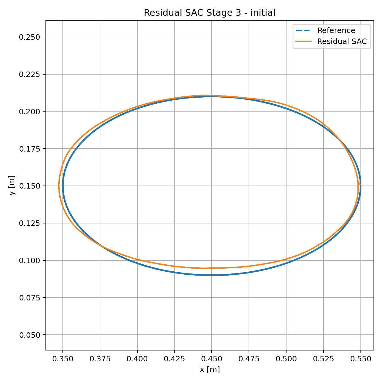
The residual architecture keeps the mismatched CTC as the baseline controller and asks SAC to learn only a bounded correction:

τ_total = τ_CTC,wrong + Δτ_SAC

Residual limits of [5, 2] Nm are selected from the measured analytical deficit with additional margin. This gives the learned policy enough authority to correct the missing dynamics while keeping the classical controller responsible for the dominant structure of the task.

Residual SAC Stage 3 initial trajectory — **Figure 8 — Residual SAC After 50k Steps**The residual policy already recovers most of the mismatch-induced error, reaching 2.956 mm Cartesian RMSE.

Residual SAC Stage 3 final trajectory — **Figure 9 — Final Residual SAC Policy**The selected 100k-step policy reaches 1.290 mm RMSE, 2.226 mm maximum error, and 97.658% geometric IoU with no actuator saturation.

5. Did the Policy Learn the Missing Physics?

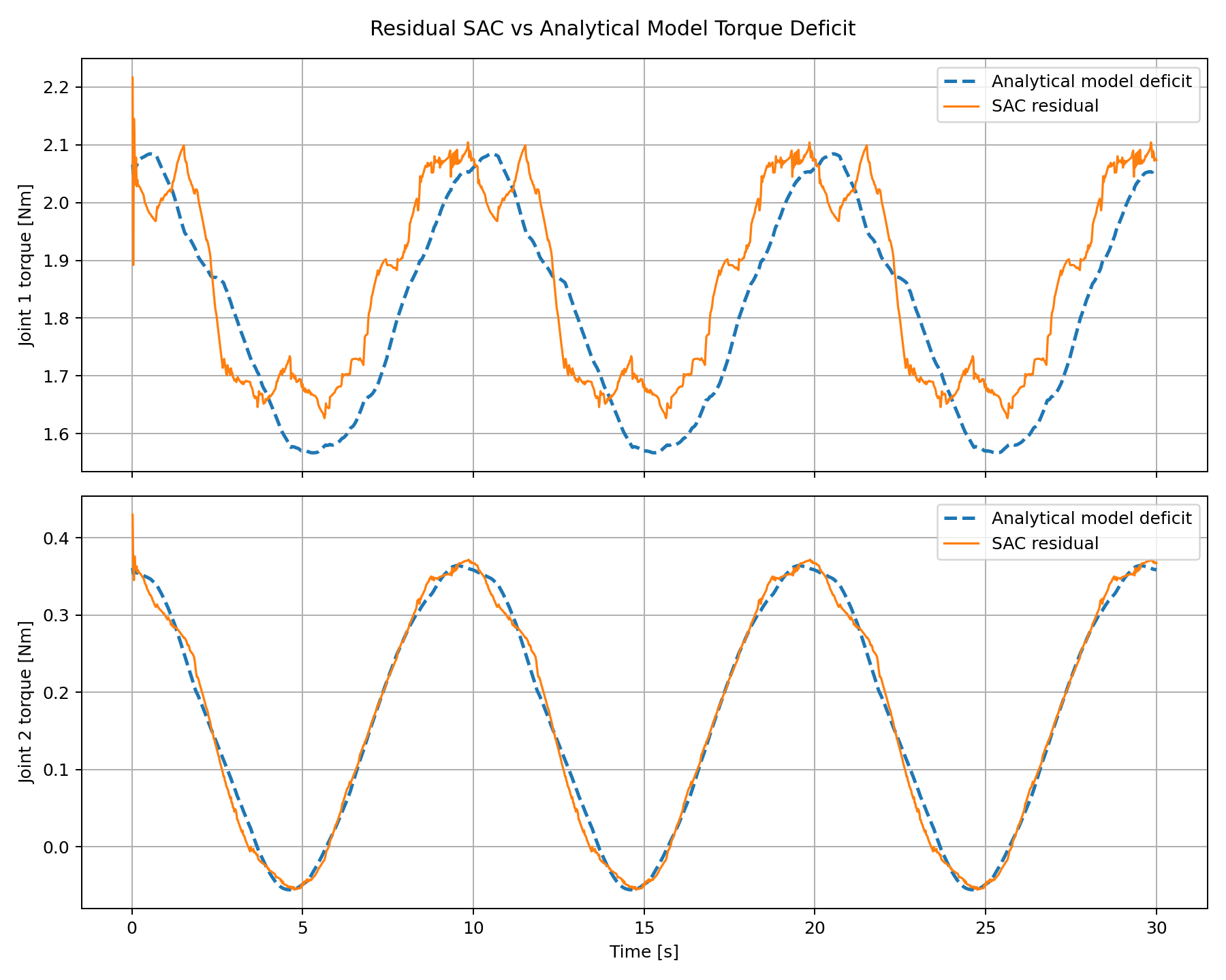
Trajectory accuracy alone cannot answer this question. The final residual torque is therefore compared at the same actual state and reference against the analytical torque deficit created by the wrong dynamics model. This is the main physical interpretation step of the project.

Final residual SAC torque compared with analytical model torque deficit — **Figure 10 — Learned Residual vs. Analytical Model Deficit**Joint 2 is reproduced almost directly, while joint 1 captures the dominant temporal structure with some remaining amplitude and phase error.

Metric	Joint 1	Joint 2
Residual-deficit RMSE	0.0978 Nm	0.0140 Nm
Residual-deficit correlation	0.880	0.996

Key interpretation: the residual policy does not merely reduce Cartesian error. Its learned correction is strongly aligned with the torque that the analytical model says is missing, supporting the interpretation that the policy is compensating a physically identifiable model deficit.

6. Final Controller Comparison

Controller	EE RMSE	Max error	Geometric error	IoU
Exact-model CTC	0.195 mm	0.278 mm	—	—
CTC, 30% link-2 mass error	31.116 mm	39.161 mm	62.230%	53.919%
Pure SAC	4.662 mm	9.930 mm	6.230%	93.994%
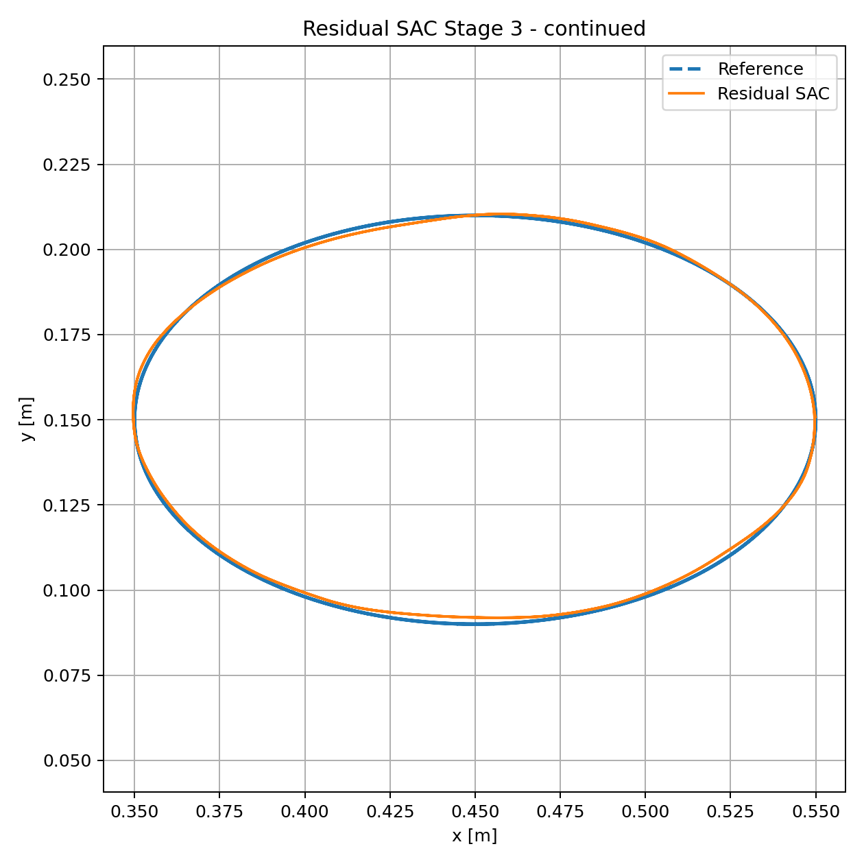
Residual SAC	1.290 mm	2.226 mm	2.353%	97.658%

What Classical Control Shows

When the analytical model is correct, computed-torque control remains the strongest solution in this benchmark. Learning is not needed simply because it is available.

What Learning Adds

When the model is deliberately wrong, learning provides value. Residual SAC is especially effective because it preserves the known control structure and learns a smaller correction problem.

7. Refinement and Stopping Decision

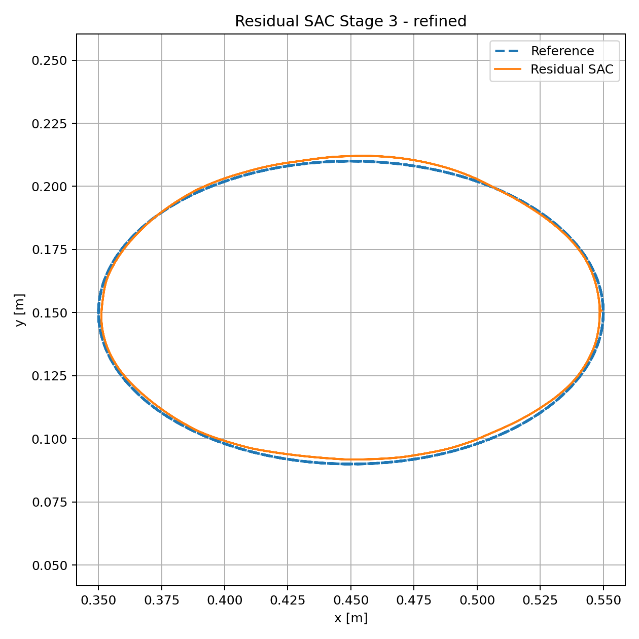
After the 100k-step residual policy reached the best measured result, the learning rate was reduced from 3×10⁻⁴ to 1×10⁻⁴ for an additional 30k steps. Performance did not improve: RMSE increased to 1.530 mm and IoU fell to 96.749%. The 100k policy was therefore retained rather than assuming that more training must be better.

Residual SAC low-learning-rate refinement trajectory — **Figure 11 — Low-Learning-Rate Refinement**Additional optimization does not improve the already-converged policy, providing a practical stopping criterion.

8. Why These Metrics?

Tracking Accuracy

End-effector RMSE and maximum error quantify typical and worst-case Cartesian tracking behavior.

Geometric Fidelity

Area bias, symmetric-difference area, geometric error, and IoU reveal closed-path distortion that RMSE alone can hide.

Control Effort

Torque RMS, peak torque, and saturation distinguish a controller error from a simple lack of actuator authority.

Physical Interpretation

Residual-deficit RMSE and correlation test whether the learned correction is consistent with the actual model error.

9. Practical Limitations

The study uses controlled simulation so that one model error can be isolated and interpreted.
Real manipulators introduce simultaneous mass, inertia, center-of-mass, friction, drivetrain, payload, and compliance uncertainty.
Sensor noise, state-estimation error, communication delay, actuator dynamics, and torque-estimation error are not modeled here.
The final policies are evaluated on the Stage-3 task distribution; broader trajectory generalization requires separate testing.
Free-space tracking does not establish robustness to contact or arbitrary external disturbance.
The exact-model CTC result is an ideal model-consistency reference, not a hardware-level accuracy prediction.

Scope of the conclusion: this project establishes a physically interpretable simulation result—model mismatch creates a measurable torque deficit, and a bounded residual policy can learn a correction strongly aligned with that deficit. Hardware robustness and sim-to-real performance remain separate validation problems.

10. Project Resources

Source & Results

Manipulator models, CTC implementation, Pure SAC and Residual SAC environments, curriculum / transfer / continuation scripts, evaluation tools, tests, and selected experiment results.

Open GitHub Project

Technical Report

Detailed report covering the control formulation, training logic, evaluation metrics, analytical torque-deficit comparison, quantitative results, physical interpretation, and real-world limitations.

View Technical Report Download PDF

← Previous: Path Planning Back to Projects →

Project by Sooyong Kim · Robotics & Autonomous Systems Portfolio